Homework 1: Quarto, Basic Syntax and Data Importing
Spring 2025 MATH/COSC 3570 Introduction to Data Science by Dr. Cheng-Han Yu
Author
Insert Your Name!!
Published
May 1, 2025
1 Autobiography
Please introduce yourself. You can share anything, your hometown, major, family, hobbies, working experience, honors and awards, special skills, etc, yes anything! Your autobiography should include:
At least two paragraphs (Paragraphs are separated by a blank line)
Bold text
Italic text
Text with both bold AND italic font (Not mentioned in class, but you should be able to figure it out)
Use the chunk option results in the chunk labelled cat, so that the text output is “I love Marquette and Data Science!”.
cat("I love **Marquette** and *Data Science*!\n")
I love **Marquette** and *Data Science*!
We can re-use a code chunk by using its name! Please use the option #| label: photo and make the empty code chunk run the code in the code chunk named photo. Note that the chunk options are not carried.
3 Basic R
3.1 Vector
Use the built-in data set LakeHuron that records annual measurements of the level, in feet, of Lake Huron 1875–1972.
Return a logical vector that shows whether the lake level is higher than the average level or not.
Return years that have a level higher than the average.
3.2 Data Frame
Make the mtcars dataset as a tibble using as_tibble(). Call it tbl.
Print the sub data of tbl that contains the 11th to 15th rows and the last three columns.
Grab the second and the third columns of tbl.
Extract the fourth column of tbl as a numerical vector.
Start with tbl, use the pipe operator |> to do the followings sequentially.
extract the first 10 observations (rows) using head()
find the column names colnames()
sort the columns names using sort() in a decreasing order. (alphabetically from z to a)
3.3 Data Importing
Use readxl::read_excel() to read the data sales.xlsx in the data folder. Use arguments sheet, skip and col_names so that the output looks like
# A tibble: 9 x 2
  id      n
  <chr>   <chr>
1 Brand 1 n
2 1234    8
3 8721    2
4 1822    3
5 Brand 2 n
6 3333    1
# … with 3 more rows
Use readxl::read_excel() to read in the favourite-food.xlsx file in the data folder and call the data fav_food. Use the argument na to treat “N/A” and “99999” as a missing value. Print the data out.
4 Basic Python
import numpy as npimport pandas as pd
4.1 Pandas Data Frame
Import the data set mtcars.csv using pd.read_csv(). Then print the first five rows.
Use method .iloc to obtain the first and fourth rows, and the second and third columns. Name the data dfcar.
Set the row names of dfcar to Mazda and Hornet.
Use method .loc to obtain row Hornet and column disp.
Use NumPy methods to create an array equivalent to mat. Call it mat_py.
Subset the mat_py so that the result is equivalent to mat[c(1, 3), 1].
Create an array equivalent to mat_c. Call it mat_py_c. Then combine them by columns using np.hstack().
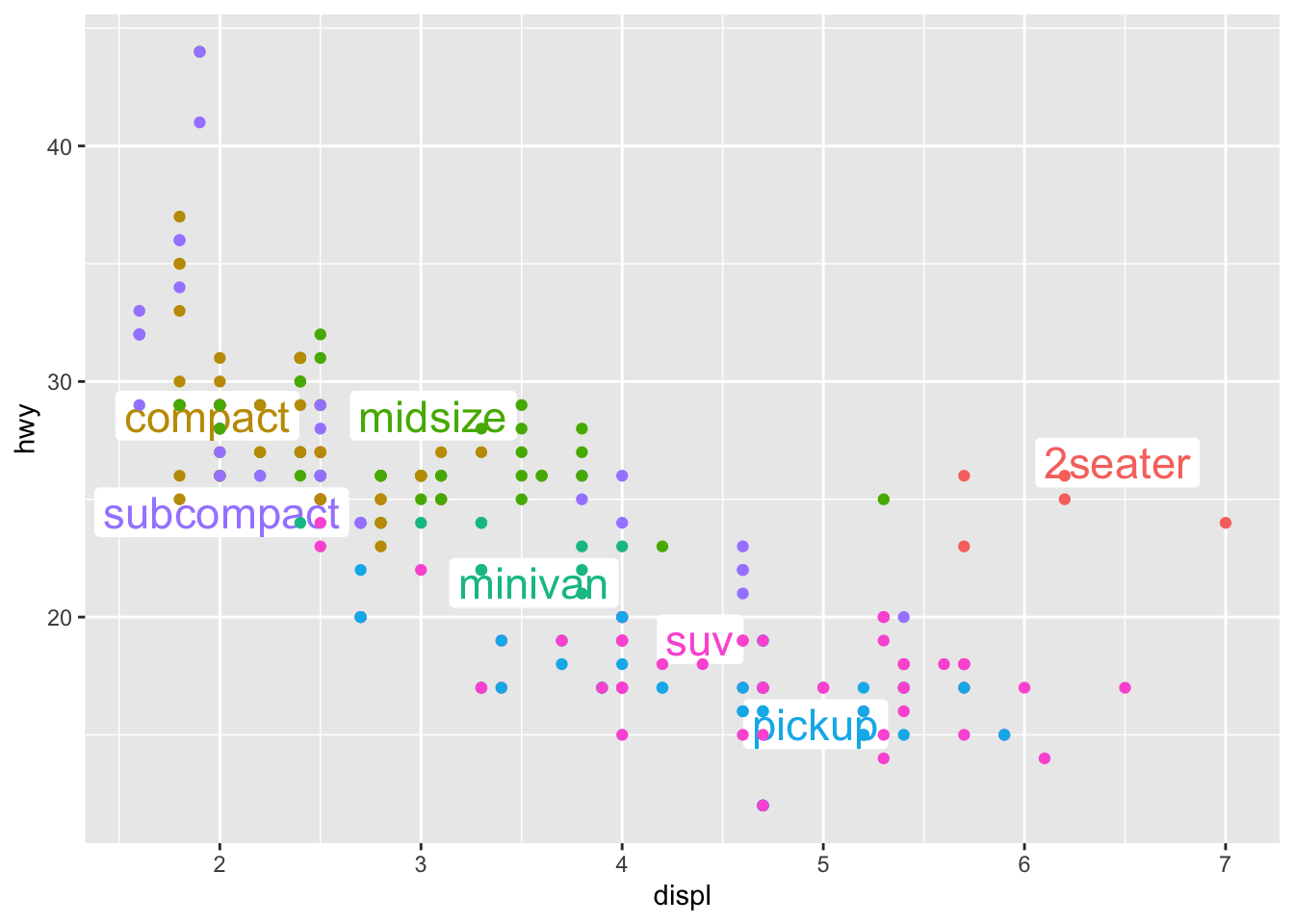
Source Code
---title: "Homework 1: Quarto, Basic Syntax and Data Importing"subtitle: "Spring 2025 MATH/COSC 3570 Introduction to Data Science by Dr. Cheng-Han Yu"format: html: code-fold: false code-tools: true toc: true toc-depth: 3date: todayauthor: "**Insert Your Name!!**"number-sections: trueeditor: source---```{r}#| label: setup#| include: false###################################################### !!!DO NOT MAKE ANY CHANGE OF THIS CODE CHUNK!!!######################################################pkgs <-c("knitr","rmarkdown", "tidyverse", "reticulate", "readxl", "ggplot2", "ggrepel", "formatR")lapply(pkgs, require, character.only =TRUE)```# Autobiography(@) Please introduce yourself. You can share anything, your hometown, major, family, hobbies, working experience, honors and awards, special skills, etc, yes anything! Your autobiography should include: - At least two paragraphs (Paragraphs are separated by a blank line) - Bold text - Italic text - Text with both bold AND italic font (Not mentioned in class, but you should be able to figure it out) - Clickable text with a hyperlink - Blockquote - Listed items - emoji To make your emoji works, add [`from: markdown+emoji`](https://quarto.org/docs/visual-editor/content.html#emojis) in your YAML header, like ``` --- title: "My Document" from: markdown+emoji --- ``` Then add emoji to your writing by typing `:EMOJICODE:`. Check [emoji cheatsheet](https://github.com/ikatyang/emoji-cheat-sheet/blob/master/README.md).**Your Self-Introduction:**# Chunk OptionsPlease check the references <https://quarto.org/docs/reference/cells/cells-knitr.html> and answer the following questions.(@) Please add your nice picture using `knitr::include_graphics()` in the code chunk labeled <ins>photo</ins>. Please use i) `echo` to not to show the code ii) `fig-cap` to add a figure caption iii) `fig-cap-location` to put the caption on the margin.```{r}#| label: photo```(@) In the code chunk <ins>opt-echo</ins>, use the chunk option i) `echo` to **NOT** to show `library(tidyverse)`, `library(ggplot2)`, and `library(ggrepel)`. *Note: you may need to use !expr. Check [stackoverflow discussion](https://stackoverflow.com/questions/72217651/quarto-rmarkdown-code-block-to-only-display-certain-lines) and [Quarto chunk options](https://quarto.org/docs/computations/r.html#chunk-options)*. ii) `fig-align` to have the figure right-aligned. ```{r} #| label: opt-echo library(tidyverse) library(ggplot2) class_avg <- mpg |> group_by(class) |> summarise(displ = median(displ), hwy = median(hwy)) library(ggrepel) ggplot(mpg, aes(displ, hwy, colour = class)) + geom_label_repel(aes(label = class), data = class_avg, size = 6, label.size = 0, segment.color = NA) + geom_point() + theme(legend.position = "none") ```(@) A Marquette student has a really bad code style. Please i) Add the chunk option `tidy` in the chunk labelled <ins>style</ins> to make her code below more readable. ii) Add another option `eval` so that the code is **NOT** run. You may need to install the package `formatR` so that the tidy format can work.```{r}#| label: stylefor(k in1:10){j=cos(sin(k)*k^2)+3;l=exp(k-7*log(k,base=2));print(j*l-5)}```(@) Use the chunk option `results` in the chunk labelled <ins>cat</ins>, so that the text output is "I love **Marquette** and *Data Science*!".```{r}#| label: catcat("I love **Marquette** and *Data Science*!\n")```(@) We can re-use a code chunk by using its name! Please use the option `#| label: photo` and make the empty code chunk run the code in the code chunk named <ins>photo</ins>. Note that the chunk options are not carried.```{r}```# Basic R## VectorUse the built-in data set `LakeHuron` that records annual measurements of the level, in feet, of Lake Huron 1875–1972.(@) Return a logical vector that shows whether the lake level is higher than the average level or not.```{r}#| label: vec-1```(@) Return years that have a level higher than the average.```{r}#| label: vec-2```## Data Frame(@) Make the `mtcars` dataset as a tibble using `as_tibble()`. Call it `tbl`.```{r}#| label: df-1```(@) Print the sub data of `tbl` that contains the 11th to 15th rows and the last three columns.```{r}#| label: df-2```(@) Grab the second and the third columns of `tbl`.```{r}#| label: df-3```(@) Extract the fourth column of `tbl` as a numerical vector.```{r}#| label: df-4```(@) Start with `tbl`, use the pipe operator `|>` to do the followings sequentially. i. extract the first 10 observations (rows) using `head()` ii. find the column names `colnames()` iii. sort the columns names using `sort()` in a *decreasing* order. (alphabetically from z to a)```{r}#| label: df-5```## Data Importing(@) Use `readxl::read_excel()` to read the data `sales.xlsx` in the data folder. Use arguments `sheet`, `skip` and `col_names` so that the output looks like # A tibble: 9 x 2 id n <chr> <chr> 1 Brand 1 n 2 1234 8 3 8721 2 4 1822 3 5 Brand 2 n 6 3333 1 # … with 3 more rows```{r}#| label: import-1```(@) Use `readxl::read_excel()` to read in the `favourite-food.xlsx` file in the data folder and call the data `fav_food`. Use the argument `na` to treat "N/A" and "99999" as a missing value. Print the data out.```{r}#| label: import-2```# Basic Python```{python}import numpy as npimport pandas as pd```## Pandas Data Frame(@) Import the data set `mtcars.csv` using `pd.read_csv()`. Then print the first five rows.```{python}#| label: pd-1```(@) Use method `.iloc` to obtain the first and fourth rows, and the second and third columns. Name the data `dfcar`.```{python}#| label: pd-2```(@) Set the row names of `dfcar` to `Mazda` and `Hornet`.```{python}#| label: pd-3```(@) Use method `.loc` to obtain row `Hornet` and column `disp`.```{python}#| label: py-4```## NumPy ArrayIn class, we learned the R data structure matrix:```{r}#| eval: falsemat <-matrix(data =1:6, nrow =3, ncol =2)mat[c(1, 3), 1] mat_c <-matrix(data =c(7, 0, 0, 8, 2, 6), nrow =3, ncol =2)cbind(mat, mat_c) ```(@) Use NumPy methods to create an array equivalent to `mat`. Call it `mat_py`.```{python}#| label: np-1```(@) Subset the `mat_py` so that the result is equivalent to `mat[c(1, 3), 1]`.```{python}#| label: np-2```(@) Create an array equivalent to `mat_c`. Call it `mat_py_c`. Then combine them by columns using `np.hstack()`.```{python}#| label: np-3```