x <- 4; y <- 3
bar <- ggplot(data = diamonds) +
  geom_bar(mapping = aes(x = cut, fill = cut),
           show.legend = FALSE, width = 1) +
  theme(aspect.ratio = 1) +
  labs(x = NULL, y = NULL)
bar + coord_flip()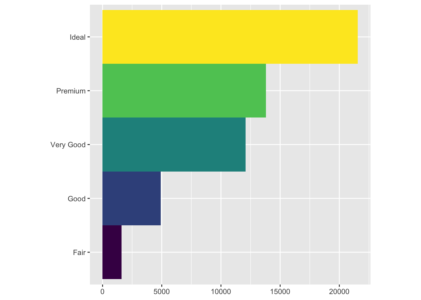
bar + coord_polar()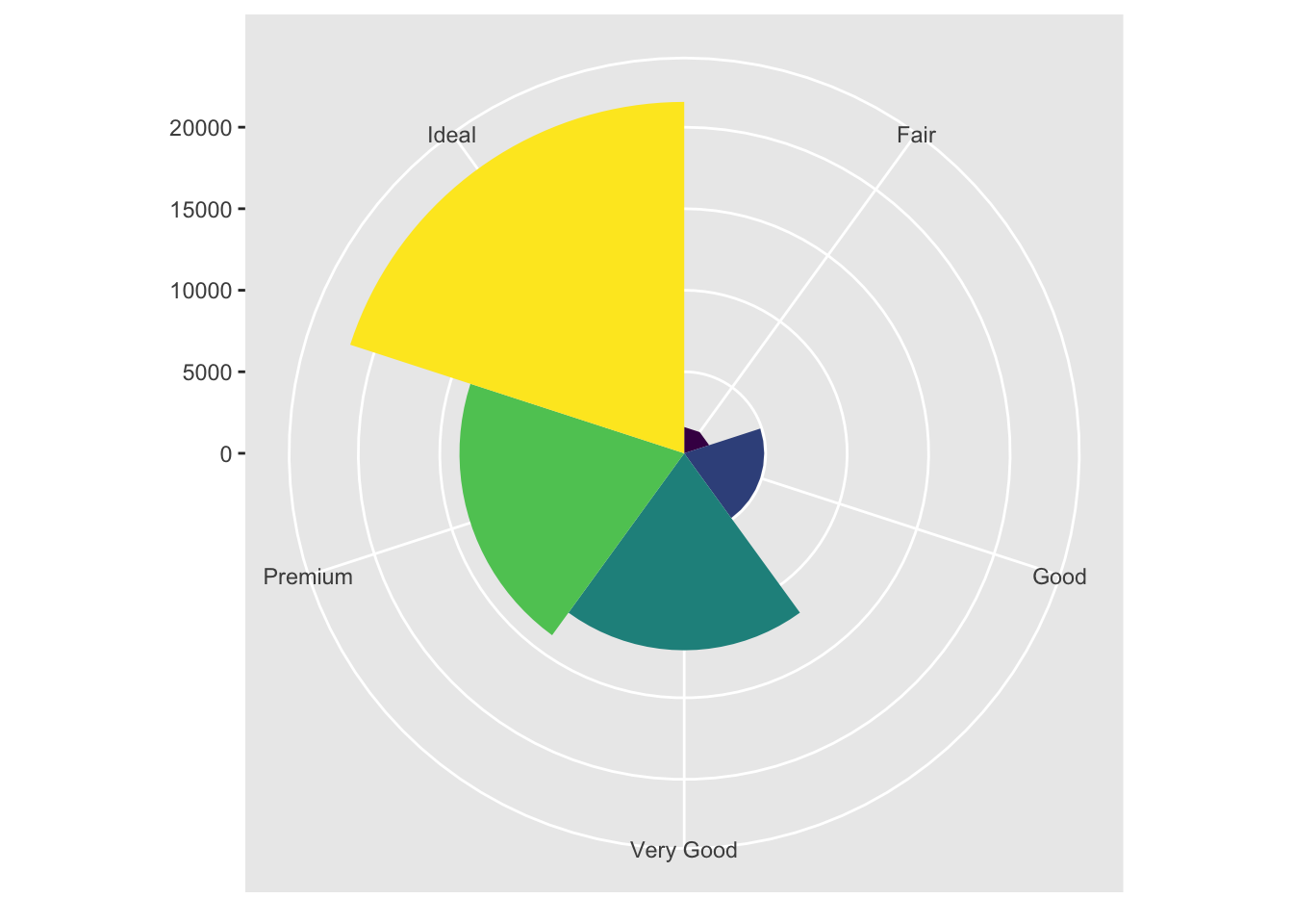
MATH/COSC 3570 Spring 2025
x <- 4; y <- 3
bar <- ggplot(data = diamonds) +
geom_bar(mapping = aes(x = cut, fill = cut),
show.legend = FALSE, width = 1) +
theme(aspect.ratio = 1) +
labs(x = NULL, y = NULL)
bar + coord_flip()
bar + coord_polar()
Briefly describe how we produce a pdf.
Hello everyone, I am Cheng-Han Yu, an assistant professor at Marquette University. I love data science!
My main research interests include
My favorite quote is
All models are wrong, but some are useful. George Box
Here I write a simple math equation \(\frac{-b \pm \sqrt{b^2 - 4ac}}{2a}\).
# include image
knitr::include_graphics("https://raw.githubusercontent.com/rstudio/hex-stickers/master/PNG/ggplot2.png")
# include plot
plot(x = mtcars$disp, y = mtcars$mpg)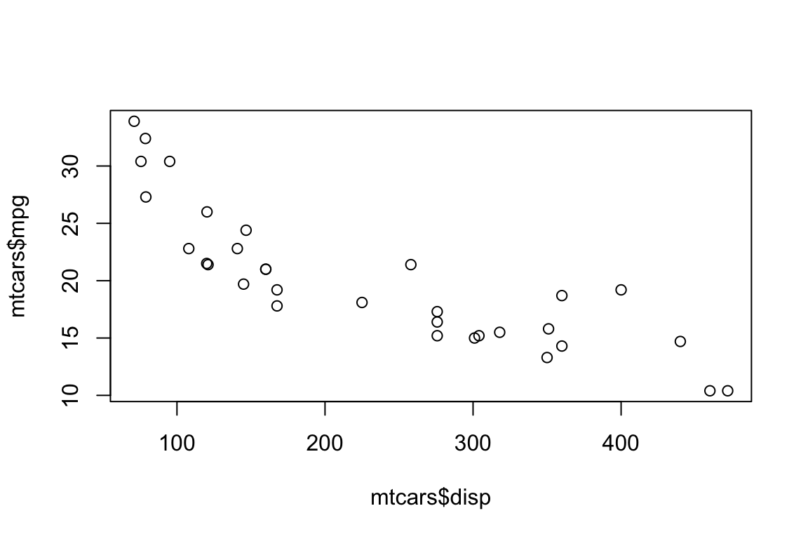
# show dataset `mtcars`
knitr::kable(mtcars, caption = "A knitr kable table of mtcars data set")| mpg | cyl | disp | hp | drat | wt | qsec | vs | am | gear | carb | |
|---|---|---|---|---|---|---|---|---|---|---|---|
| Mazda RX4 | 21.0 | 6 | 160.0 | 110 | 3.90 | 2.620 | 16.46 | 0 | 1 | 4 | 4 |
| Mazda RX4 Wag | 21.0 | 6 | 160.0 | 110 | 3.90 | 2.875 | 17.02 | 0 | 1 | 4 | 4 |
| Datsun 710 | 22.8 | 4 | 108.0 | 93 | 3.85 | 2.320 | 18.61 | 1 | 1 | 4 | 1 |
| Hornet 4 Drive | 21.4 | 6 | 258.0 | 110 | 3.08 | 3.215 | 19.44 | 1 | 0 | 3 | 1 |
| Hornet Sportabout | 18.7 | 8 | 360.0 | 175 | 3.15 | 3.440 | 17.02 | 0 | 0 | 3 | 2 |
| Valiant | 18.1 | 6 | 225.0 | 105 | 2.76 | 3.460 | 20.22 | 1 | 0 | 3 | 1 |
| Duster 360 | 14.3 | 8 | 360.0 | 245 | 3.21 | 3.570 | 15.84 | 0 | 0 | 3 | 4 |
| Merc 240D | 24.4 | 4 | 146.7 | 62 | 3.69 | 3.190 | 20.00 | 1 | 0 | 4 | 2 |
| Merc 230 | 22.8 | 4 | 140.8 | 95 | 3.92 | 3.150 | 22.90 | 1 | 0 | 4 | 2 |
| Merc 280 | 19.2 | 6 | 167.6 | 123 | 3.92 | 3.440 | 18.30 | 1 | 0 | 4 | 4 |
| Merc 280C | 17.8 | 6 | 167.6 | 123 | 3.92 | 3.440 | 18.90 | 1 | 0 | 4 | 4 |
| Merc 450SE | 16.4 | 8 | 275.8 | 180 | 3.07 | 4.070 | 17.40 | 0 | 0 | 3 | 3 |
| Merc 450SL | 17.3 | 8 | 275.8 | 180 | 3.07 | 3.730 | 17.60 | 0 | 0 | 3 | 3 |
| Merc 450SLC | 15.2 | 8 | 275.8 | 180 | 3.07 | 3.780 | 18.00 | 0 | 0 | 3 | 3 |
| Cadillac Fleetwood | 10.4 | 8 | 472.0 | 205 | 2.93 | 5.250 | 17.98 | 0 | 0 | 3 | 4 |
| Lincoln Continental | 10.4 | 8 | 460.0 | 215 | 3.00 | 5.424 | 17.82 | 0 | 0 | 3 | 4 |
| Chrysler Imperial | 14.7 | 8 | 440.0 | 230 | 3.23 | 5.345 | 17.42 | 0 | 0 | 3 | 4 |
| Fiat 128 | 32.4 | 4 | 78.7 | 66 | 4.08 | 2.200 | 19.47 | 1 | 1 | 4 | 1 |
| Honda Civic | 30.4 | 4 | 75.7 | 52 | 4.93 | 1.615 | 18.52 | 1 | 1 | 4 | 2 |
| Toyota Corolla | 33.9 | 4 | 71.1 | 65 | 4.22 | 1.835 | 19.90 | 1 | 1 | 4 | 1 |
| Toyota Corona | 21.5 | 4 | 120.1 | 97 | 3.70 | 2.465 | 20.01 | 1 | 0 | 3 | 1 |
| Dodge Challenger | 15.5 | 8 | 318.0 | 150 | 2.76 | 3.520 | 16.87 | 0 | 0 | 3 | 2 |
| AMC Javelin | 15.2 | 8 | 304.0 | 150 | 3.15 | 3.435 | 17.30 | 0 | 0 | 3 | 2 |
| Camaro Z28 | 13.3 | 8 | 350.0 | 245 | 3.73 | 3.840 | 15.41 | 0 | 0 | 3 | 4 |
| Pontiac Firebird | 19.2 | 8 | 400.0 | 175 | 3.08 | 3.845 | 17.05 | 0 | 0 | 3 | 2 |
| Fiat X1-9 | 27.3 | 4 | 79.0 | 66 | 4.08 | 1.935 | 18.90 | 1 | 1 | 4 | 1 |
| Porsche 914-2 | 26.0 | 4 | 120.3 | 91 | 4.43 | 2.140 | 16.70 | 0 | 1 | 5 | 2 |
| Lotus Europa | 30.4 | 4 | 95.1 | 113 | 3.77 | 1.513 | 16.90 | 1 | 1 | 5 | 2 |
| Ford Pantera L | 15.8 | 8 | 351.0 | 264 | 4.22 | 3.170 | 14.50 | 0 | 1 | 5 | 4 |
| Ferrari Dino | 19.7 | 6 | 145.0 | 175 | 3.62 | 2.770 | 15.50 | 0 | 1 | 5 | 6 |
| Maserati Bora | 15.0 | 8 | 301.0 | 335 | 3.54 | 3.570 | 14.60 | 0 | 1 | 5 | 8 |
| Volvo 142E | 21.4 | 4 | 121.0 | 109 | 4.11 | 2.780 | 18.60 | 1 | 1 | 4 | 2 |
There are 11 variables in the mtcars data set.
Answer to the questions.
radius = 5The radius of the circle is {python} print(radius)
v1 <- c(3, 8, 4, 5)
fac <- factor(c("bad", "neutral", "good"))
x_lst <- list(idx = 1:3,
              "a",
              c(TRUE, FALSE))
mat <- matrix(data = 1:6,
              nrow = 3,
              ncol = 2)
df <- data.frame(age = c(19, 21, 40),
                 gender = c("m","f", "m"))
vec <- c(type = typeof(v1), class = class(v1))
fac <- c(type = typeof(fac), class = class(fac))
lst <- c(type = typeof(x_lst), class = class(x_lst))
mat <- c(type = typeof(mat), class = class(mat))
df <- c(type = typeof(df), class = class(df))
list(vector = vec,
     factor = fac,
     list = lst,
     matrix = mat,
     dataframe = df)
$vector
type class
"double" "numeric"
$factor
type class
"integer" "factor"
$list
type class
"list" "list"
$matrix
type class1 class2
"integer" "matrix" "array"
$dataframe
type class
"list" "data.frame" x_lst <- list(idx = 1:3,
word = "a",
bool = c(TRUE, FALSE))py_lst = [[1, 2, 3], "a", [True, False]]
py_lst[[1, 2, 3], 'a', [True, False]]py_dic = {"idx": [1, 2, 3], "word": "a", "bool": [True, False]}
py_dic{'idx': [1, 2, 3], 'word': 'a', 'bool': [True, False]}plot(mtcars$mpg, mtcars$wt,
col = 4, pch = 8, cex = 2,
xlab = "MPG", ylab = "Wt. (1000 lbs)",
main = "MPG vs. Weight")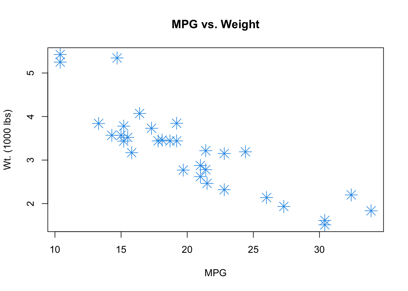
hist(mtcars$qsec, breaks = 20, border = "#FFCC00",
     col = 2, main = "Histogram of 1/4 mile time")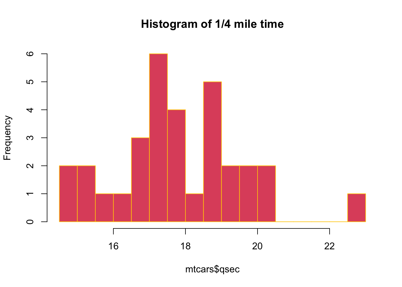
boxplot(mpg ~ gear,
        data = mtcars,
        col = 2:4,
        las = 1,
        horizontal = TRUE,
        xlab = "Miles per gallon",
        ylab = "Number of forward gears")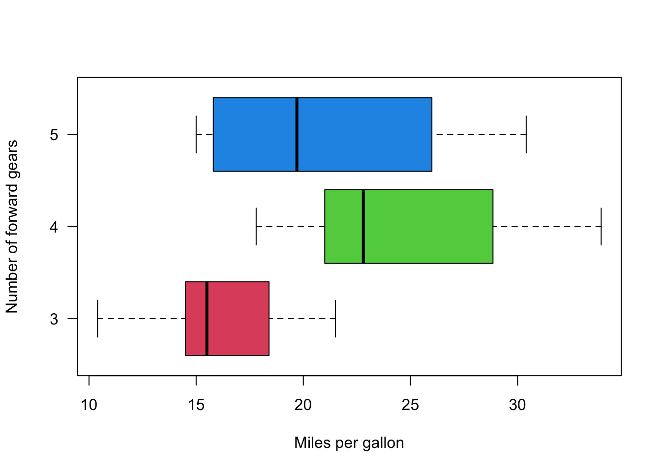
import pandas as pd
import matplotlib.pyplot as plt
mtcars = pd.read_csv('./data/mtcars.csv')
mtcars
mpg cyl disp hp drat wt qsec vs am gear carb
0 21.0 6 160.0 110 3.90 2.620 16.46 0 1 4 4
1 21.0 6 160.0 110 3.90 2.875 17.02 0 1 4 4
2 22.8 4 108.0 93 3.85 2.320 18.61 1 1 4 1
3 21.4 6 258.0 110 3.08 3.215 19.44 1 0 3 1
4 18.7 8 360.0 175 3.15 3.440 17.02 0 0 3 2
5 18.1 6 225.0 105 2.76 3.460 20.22 1 0 3 1
6 14.3 8 360.0 245 3.21 3.570 15.84 0 0 3 4
7 24.4 4 146.7 62 3.69 3.190 20.00 1 0 4 2
8 22.8 4 140.8 95 3.92 3.150 22.90 1 0 4 2
9 19.2 6 167.6 123 3.92 3.440 18.30 1 0 4 4
10 17.8 6 167.6 123 3.92 3.440 18.90 1 0 4 4
11 16.4 8 275.8 180 3.07 4.070 17.40 0 0 3 3
12 17.3 8 275.8 180 3.07 3.730 17.60 0 0 3 3
13 15.2 8 275.8 180 3.07 3.780 18.00 0 0 3 3
14 10.4 8 472.0 205 2.93 5.250 17.98 0 0 3 4
15 10.4 8 460.0 215 3.00 5.424 17.82 0 0 3 4
16 14.7 8 440.0 230 3.23 5.345 17.42 0 0 3 4
17 32.4 4 78.7 66 4.08 2.200 19.47 1 1 4 1
18 30.4 4 75.7 52 4.93 1.615 18.52 1 1 4 2
19 33.9 4 71.1 65 4.22 1.835 19.90 1 1 4 1
20 21.5 4 120.1 97 3.70 2.465 20.01 1 0 3 1
21 15.5 8 318.0 150 2.76 3.520 16.87 0 0 3 2
22 15.2 8 304.0 150 3.15 3.435 17.30 0 0 3 2
23 13.3 8 350.0 245 3.73 3.840 15.41 0 0 3 4
24 19.2 8 400.0 175 3.08 3.845 17.05 0 0 3 2
25 27.3 4 79.0 66 4.08 1.935 18.90 1 1 4 1
26 26.0 4 120.3 91 4.43 2.140 16.70 0 1 5 2
27 30.4 4 95.1 113 3.77 1.513 16.90 1 1 5 2
28 15.8 8 351.0 264 4.22 3.170 14.50 0 1 5 4
29 19.7 6 145.0 175 3.62 2.770 15.50 0 1 5 6
30 15.0 8 301.0 335 3.54 3.570 14.60 0 1 5 8
31 21.4 4 121.0 109 4.11 2.780 18.60 1 1 4 2plt.scatter(x = mtcars.mpg,
y = mtcars.wt,
color = "r")
plt.xlabel("Miles per gallon")
plt.ylabel("Weight")
plt.title("Scatter plot")
plt.show()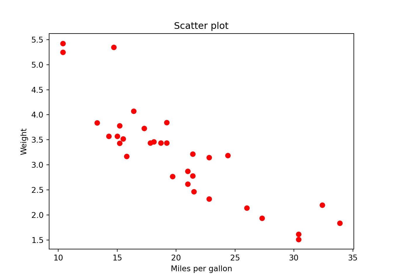
plt.clf()
plt.hist(mtcars.qsec,
         bins = 19,
         color="#003366",
         edgecolor="#FFCC00")
plt.xlabel("1/4 mile time")
plt.title("Histogram of 1/4 mile time")
plt.show()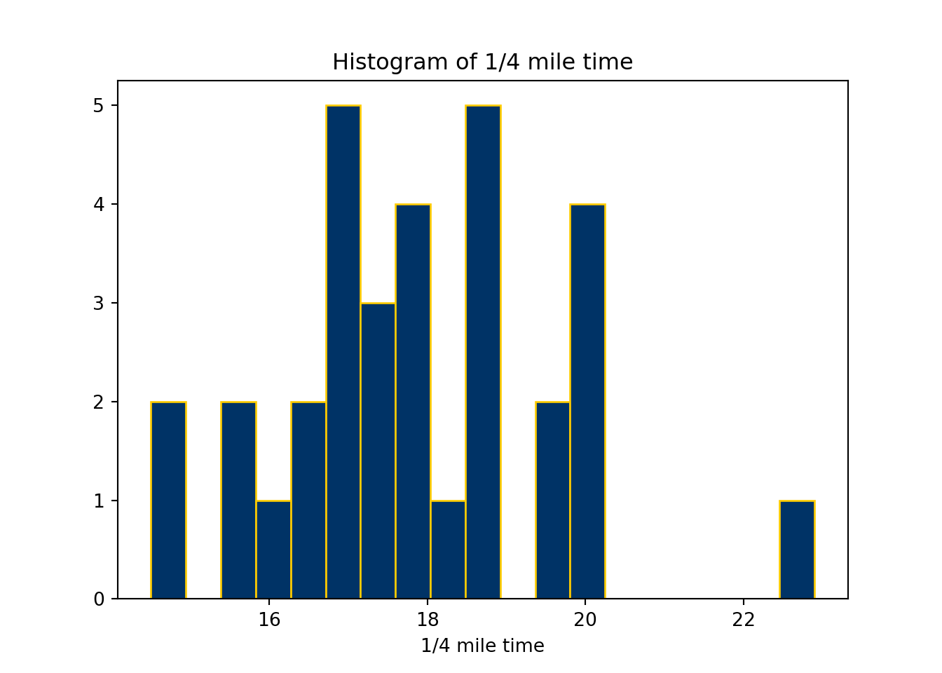
df <- data.frame(abc = 1:2,
                 xyz = c("a", "b"))
# list method
df$x
[1] "a" "b"df[[2]][1] "a" "b"df["xyz"] xyz
1 a
2 bdf[c("abc", "xyz")] abc xyz
1 1 a
2 2 b# matrix method
df[, 2][1] "a" "b"df[, "xyz"][1] "a" "b"df[, c("abc", "xyz")] abc xyz
1 1 a
2 2 blibrary(tidyverse)── Attaching core tidyverse packages ──────────────────────── tidyverse 2.0.0 ──
✔ dplyr 1.1.4 ✔ readr 2.1.5
✔ forcats 1.0.0 ✔ stringr 1.5.1
✔ lubridate 1.9.3 ✔ tibble 3.2.1
✔ purrr 1.0.2 ✔ tidyr 1.3.1
── Conflicts ────────────────────────────────────────── tidyverse_conflicts() ──
✖ dplyr::filter() masks stats::filter()
✖ dplyr::lag() masks stats::lag()
ℹ Use the conflicted package (<http://conflicted.r-lib.org/>) to force all conflicts to become errorstib <- tibble(abc = 1:2,
xyz = c("a", "b"))
# list method
tib$xWarning: Unknown or uninitialised column: `x`.NULLtib[[2]][1] "a" "b"tib["xyz"]# A tibble: 2 × 1
xyz
<chr>
1 a
2 b tib[c("abc", "xyz")]# A tibble: 2 × 2
abc xyz
<int> <chr>
1 1 a
2 2 b # matrix method
tib[, 2]# A tibble: 2 × 1
xyz
<chr>
1 a
2 b tib[, "xyz"]# A tibble: 2 × 1
xyz
<chr>
1 a
2 b tib[, c("abc", "xyz")]# A tibble: 2 × 2
abc xyz
<int> <chr>
1 1 a
2 2 b Explain their differences.
With data.frames,
$ operator will match any column name that starts with the name following it. Since there is a column named xyz, the expression df$x will be expanded to df$xyz. This behavior of the $ operator saves a few keystrokes, but it can result in accidentally using a different column than you thought you were using.[ the type of object that is returned differs on the number of columns. If it is one column, it won’t return a data.frame, but instead will return a vector. With more than one column, then it will return a data.frame. This is fine if you know what you are passing in, but suppose you did df[ , vars] where vars was a variable. Then what that code does depends on length(vars) and you’d have to write code to account for those situations or risk bugs.For tibbles,
When using the matrix subsetting method, a tibble always return a tibble.
When using $ to grab an element, tibbles never do partial matching.
[]always returns another tibble, regardless of list or matrix subsetting method.
$and[[]]return a vector.
Tibbles never do partial matching and name “x” cannot be recognized.
What does tibble::enframe() do? Try enframe(c(a = 1, b = 2, c = 3)). Check ?enframe for more details.
The function tibble::enframe() converts named vectors to a data frame with names and values
iris |> tail(n = 12) |> summary() Sepal.Length Sepal.Width Petal.Length Petal.Width
Min. :5.800 Min. :2.500 Min. :4.800 Min. :1.800
1st Qu.:6.150 1st Qu.:3.000 1st Qu.:5.100 1st Qu.:1.900
Median :6.600 Median :3.050 Median :5.200 Median :2.200
Mean :6.450 Mean :3.033 Mean :5.292 Mean :2.133
3rd Qu.:6.725 3rd Qu.:3.125 3rd Qu.:5.450 3rd Qu.:2.300
Max. :6.900 Max. :3.400 Max. :5.900 Max. :2.500
Species
setosa : 0
versicolor: 0
virginica :12
tibble(x = 1:5, y = 5:1, z = LETTERS[1:5])# A tibble: 5 × 3
x y z
<int> <int> <chr>
1 1 5 A
2 2 4 B
3 3 3 C
4 4 2 D
5 5 1 E import numpy as np
import pandas as pd
import string
list(string.ascii_uppercase)['A', 'B', 'C', 'D', 'E', 'F', 'G', 'H', 'I', 'J', 'K', 'L', 'M', 'N', 'O', 'P', 'Q', 'R', 'S', 'T', 'U', 'V', 'W', 'X', 'Y', 'Z']dic = {'x':np.arange(1, 6), 'y': np.arange(5, 0, -1), 'z':list(string.ascii_uppercase)[0:5]}
pd.DataFrame(dic) x y z
0 1 5 A
1 2 4 B
2 3 3 C
3 4 2 D
4 5 1 Elibrary(tidyverse)
# ssa <- read_csv(file = "./data/ssa-death-probability.csv")
# ssa_male <- ssa[ssa$Sex == "Male",]
# ssa_female <- ssa[ssa$Sex == "Female",]
ssa_male <- readr::read_csv("./data/ssa_male_prob.csv")Rows: 120 Columns: 5
── Column specification ────────────────────────────────────────────────────────
Delimiter: ","
chr (1): Sex
dbl (4): Age, DeathProb, NumberOfLives, LifeExp
ℹ Use `spec()` to retrieve the full column specification for this data.
ℹ Specify the column types or set `show_col_types = FALSE` to quiet this message.ssa_female <- readr::read_rds("./data/ssa_female_prob.Rds")
plot(x = ssa_female$Age, y = ssa_female$LifeExp,
type = "l", col = 2, lwd = 3,
xlab = "Age", ylab = "Life Exp",
main = "Age vs. Life Exp by Gender")
lines(ssa_male$Age, ssa_male$LifeExp, col = 4, lwd = 3) 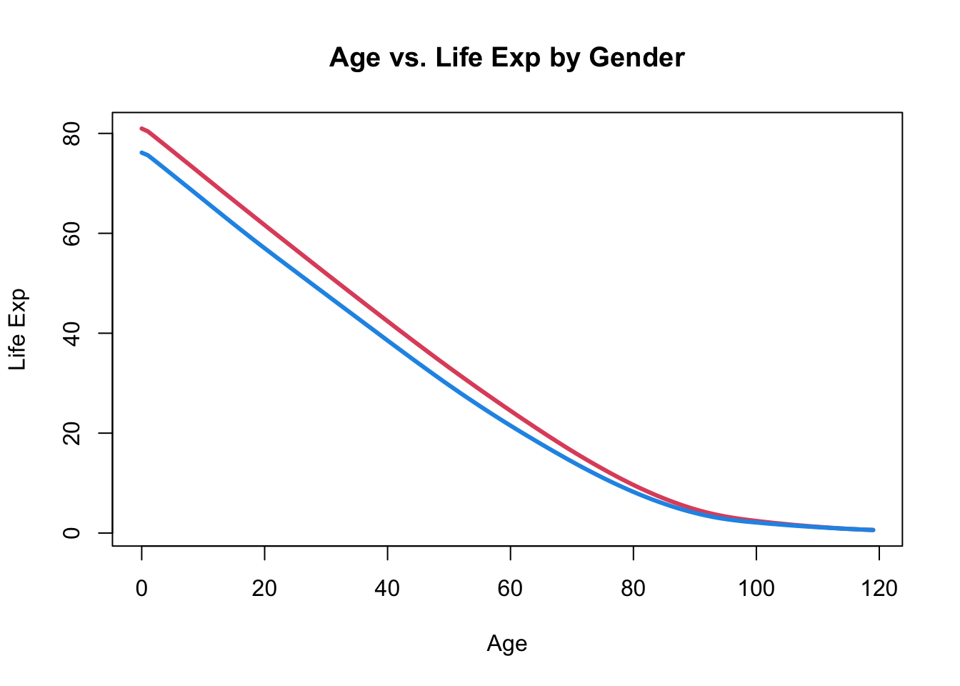
penguins <- read_csv("./data/penguins.csv")Rows: 344 Columns: 8
── Column specification ────────────────────────────────────────────────────────
Delimiter: ","
chr (3): species, island, sex
dbl (5): bill_length_mm, bill_depth_mm, flipper_length_mm, body_mass_g, year
ℹ Use `spec()` to retrieve the full column specification for this data.
ℹ Specify the column types or set `show_col_types = FALSE` to quiet this message.penguins |>
ggplot(mapping = aes(x = bill_depth_mm,
y = bill_length_mm,
colour = species)) +
geom_point() +
labs(title = "Bill depth and length",
subtitle = "Dimensions for Adelie, Chinstrap, and Gentoo Penguins",
x = "Bill depth (mm)", y = "Bill length (mm)",
colour = "Species",
caption = "Source: Palmer Station LTER / palmerpenguins package") +
scale_colour_viridis_d()Warning: Removed 2 rows containing missing values or values outside the scale range
(`geom_point()`).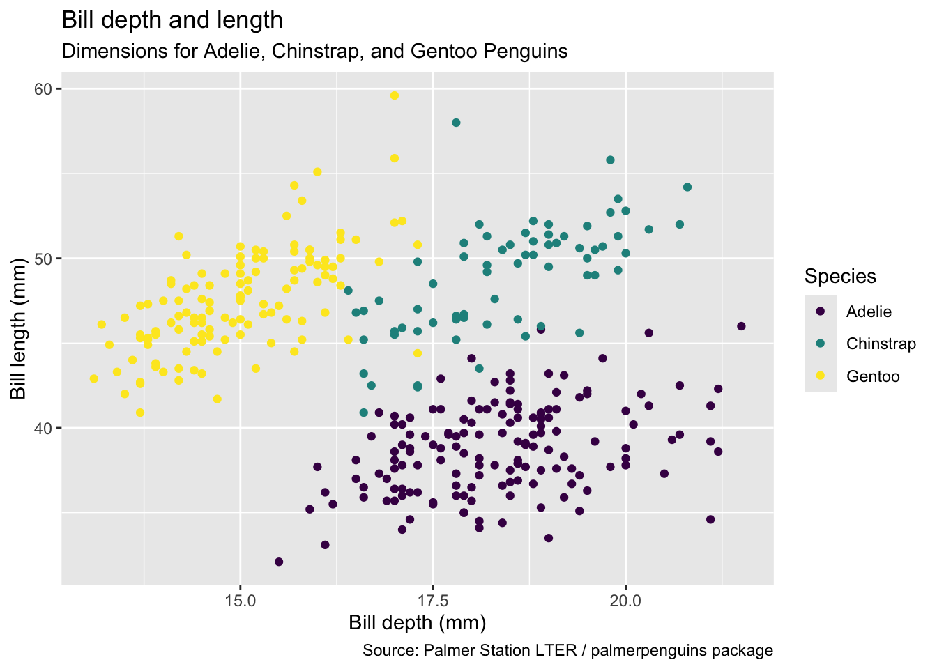
mpg |> ggplot(mapping = aes(x = displ, y = cty, color = drv, shape = fl)) +
    geom_point(size = 3, alpha = 0.8) +
    facet_grid(drv ~ fl) +
    guides(color = "none")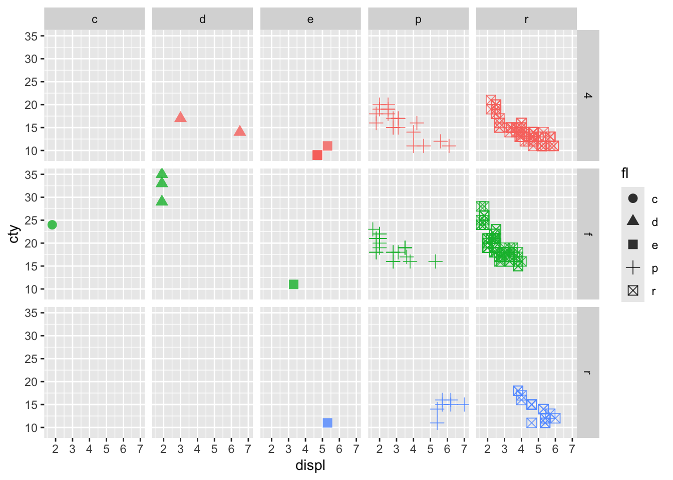
penguins <- read_csv("./data/penguins.csv")Rows: 344 Columns: 8
── Column specification ────────────────────────────────────────────────────────
Delimiter: ","
chr (3): species, island, sex
dbl (5): bill_length_mm, bill_depth_mm, flipper_length_mm, body_mass_g, year
ℹ Use `spec()` to retrieve the full column specification for this data.
ℹ Specify the column types or set `show_col_types = FALSE` to quiet this message.penguins |> ggplot(aes(x = species, fill = species)) +
geom_bar() +
labs(x = "Species of Penguins",
title = "Species Counts in Penguins Data")
penguins |> ggplot(aes(x = bill_length_mm,
                       fill = species)) +
    geom_histogram() +
    labs(x = "Bill Length (mm)",
         y = "Frequency",
         title = "Penguins Bill Length by Species") +
    facet_wrap(~ species, nrow = 1) +
    theme(legend.position = "none")
`stat_bin()` using `bins = 30`. Pick better value with `binwidth`.Warning: Removed 2 rows containing non-finite outside the scale range
(`stat_bin()`).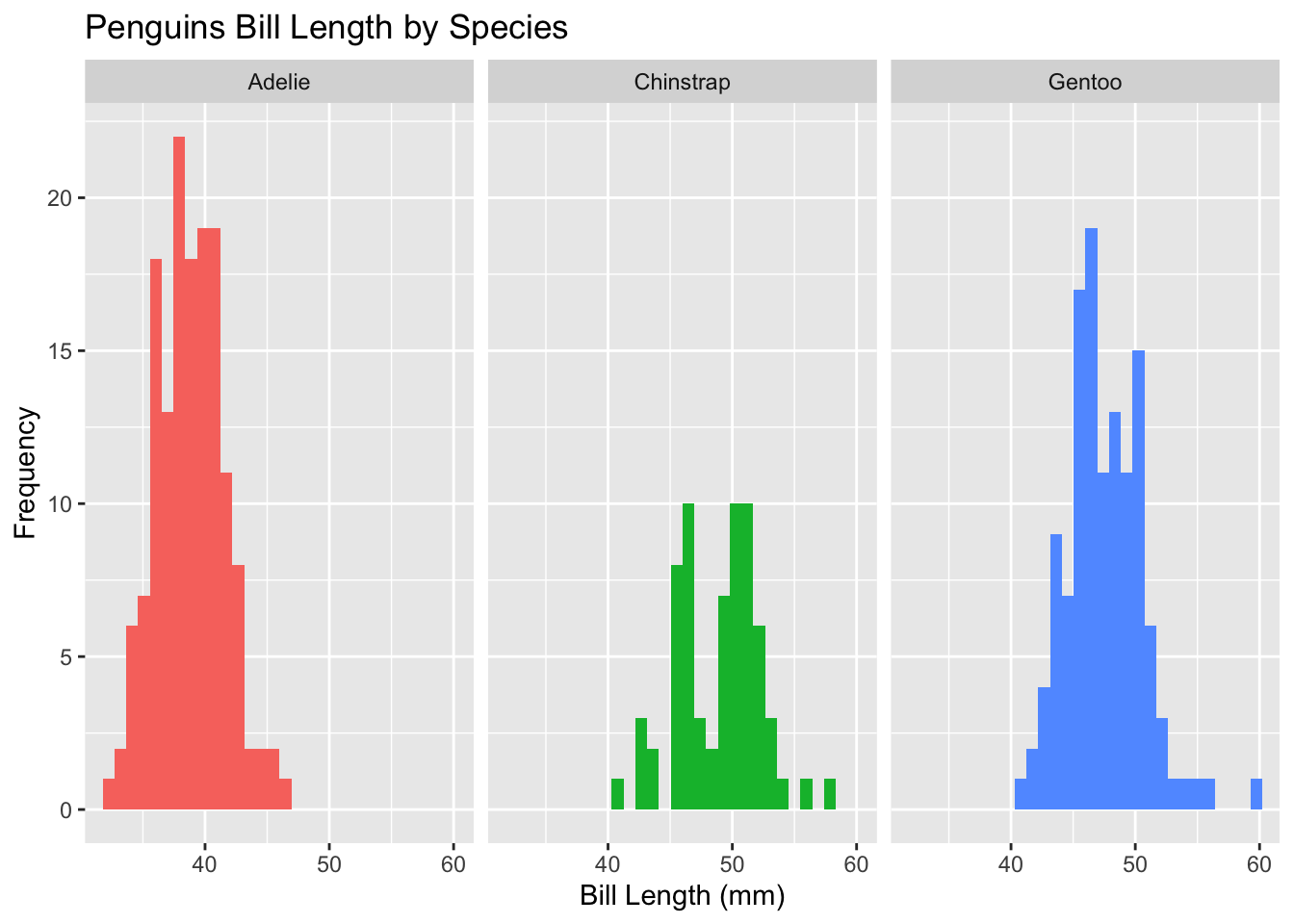
library(plotly)
Attaching package: 'plotly'The following object is masked from 'package:ggplot2':
last_plotThe following object is masked from 'package:stats':
filterThe following object is masked from 'package:graphics':
layoutloans <- readr::read_csv("./data/loans.csv")Rows: 10000 Columns: 5── Column specification ────────────────────────────────────────────────────────
Delimiter: ","
chr (2): grade, homeownership
dbl (3): loan_amount, interest_rate, debt_to_income
ℹ Use `spec()` to retrieve the full column specification for this data.
ℹ Specify the column types or set `show_col_types = FALSE` to quiet this message.p <- plot_ly(loans, x = ~interest_rate, alpha = 0.5)
p |> add_boxplot(y = ~grade, color = ~grade)# x = interest_rate, y = grade won't work
gg <- loans %>% ggplot(aes(x = grade, y = interest_rate, color = grade)) +
geom_boxplot() + theme_minimal() + coord_flip()
ggplotly(gg)murders <- read.csv("./data/murders.csv")
(my_states <- murders |>
mutate(rate = total / population * 100000) |>
filter(region %in% c("West", "Northeast"), rate < 1) |>
select(state, region, rate)) state region rate
1 Hawaii West 0.5145920
2 Idaho West 0.7655102
3 Maine Northeast 0.8280881
4 New Hampshire Northeast 0.3798036
5 Oregon West 0.9396843
6 Utah West 0.7959810
7 Vermont Northeast 0.3196211
8 Wyoming West 0.8871131my_states |>
group_by(region) |>
summarize(avg = mean(rate), std_dev = sd(rate)) |>
arrange(desc(avg))# A tibble: 2 × 3
region avg std_dev
<chr> <dbl> <dbl>
1 West 0.781 0.164
2 Northeast 0.509 0.278diamond_color <- read_csv("https://www.jaredlander.com/data/DiamondColors.csv")Rows: 10 Columns: 3
── Column specification ────────────────────────────────────────────────────────
Delimiter: ","
chr (3): Color, Description, Details
ℹ Use `spec()` to retrieve the full column specification for this data.
ℹ Specify the column types or set `show_col_types = FALSE` to quiet this message.joined_df <- left_join(diamonds, diamond_color, by = c('color' = 'Color')) |>
select(carat, color, price, Description, Details)
joined_df# A tibble: 53,940 × 5
carat color price Description Details
<dbl> <chr> <int> <chr> <chr>
1 0.23 E 326 Colorless Minute traces of color
2 0.21 E 326 Colorless Minute traces of color
3 0.23 E 327 Colorless Minute traces of color
4 0.29 I 334 Near Colorless Slightly detectable color
5 0.31 J 335 Near Colorless Slightly detectable color
6 0.24 J 336 Near Colorless Slightly detectable color
7 0.24 I 336 Near Colorless Slightly detectable color
8 0.26 H 337 Near Colorless Color is dificult to detect
9 0.22 E 337 Colorless Minute traces of color
10 0.23 H 338 Near Colorless Color is dificult to detect
# ℹ 53,930 more rowsjoined_df |> ggplot(aes(x = color)) +
geom_bar()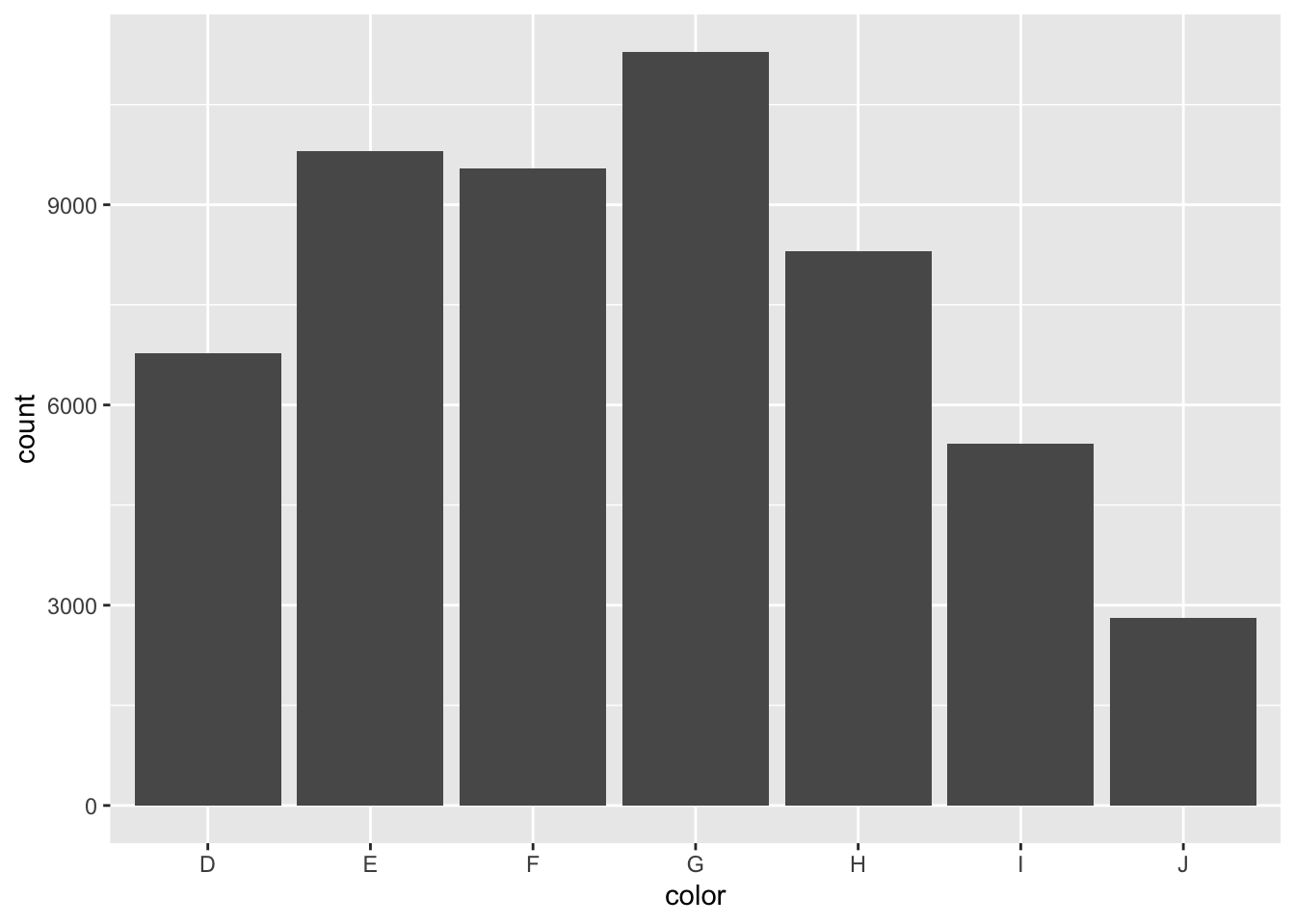
joined_df |> count(color, sort = TRUE)# A tibble: 7 × 2
color n
<chr> <int>
1 G 11292
2 E 9797
3 F 9542
4 H 8304
5 D 6775
6 I 5422
7 J 2808