Tidying Data 🧹

MATH/COSC 3570 Introduction to Data Science

Dr. Cheng-Han Yu
Department of Mathematical and Statistical Sciences
Marquette University

Grammar of Data Tidying

• OK. We are still in the stage of data wrangling. But here we are gonna tidy our data using another tidyverse package called tidyr.

Grammar of Data Tidying

• Have data organised in an unideal way for our analysis

• Want to re-organise the data to carry on with our analysis

The goal of tidyr is to help you tidy your data via

• pivoting for going between wide and long data

• separating and uniting character columns

• clarifying how NAs should be treated

• nesting and unnesting columns

• Suppose we have a data set that is untidy, and organised in an unideal way for our analysis.
• What tidyr is doing is not like dplyr, just filter rows or select columns, because it is kinda meaningless, because the data after filtering or selecting from the untidy data are still untidy.
• So our goal is to re-organise the data so that it is clean enough for being filtered or selected and for later data analysis.
• tidyr helps you tidy your data via
  • pivoting for going between wide and long data
  • separating and uniting character columns
  • clarifying how NAs should be treated. for example, do we wanna keep them or drop them, or fill in with some values.
  • nesting and unnesting columns
• We will go through the first three. You can check the tidyr page to learn more about its functionality.

Wide Data

To tidy your data, (1) figure out what the (column) variables and (row) observations are; (2) resolve one of two common problems:

One (column) variable spreads across multiple columns

customers <- read_csv("./data/sales/customers.csv")

wider (\(2 \times 4\))

more columns than we want!

customers

# A tibble: 2 × 4
  customer_id item_1 item_2       item_3
        <dbl> <chr>  <chr>        <chr> 
1           1 bread  milk         banana
2           2 milk   toilet paper <NA>  

• We may want one single column variable item showing all purchased times.

Long Data

One (row) subject is scattered across multiple rows

longer (\(6 \times 3\))

more rows than we want!

# A tibble: 6 × 3
  customer_id item_no item        
        <dbl> <chr>   <chr>       
1           1 item_1  bread       
2           1 item_2  milk        
3           1 item_3  banana      
4           2 item_1  milk        
5           2 item_2  toilet paper
6           2 item_3  <NA>        

• We may want each row corresponds to one single customer, not one single purchased item.

• Which data format we adopt depends on our own research question.

• If our data is untidy, to tidy our data, first, we get to figure out what the variables (column) and observations (row) are. Remember the definition of tidy data. each row is for one and only one observation, and each column is for one and only one variable.
• Once we know observations and variables, we need to resolve one of two common problems:
  • One variable might be spread across multiple columns.
  • One observation might be scattered across multiple rows.
• either problem is a reason why our data is not tidy.

pivot_longer() and pivot_wider()

• To transform our data to the one we want, we use pivot_longer() and pivot_wider().

• Starts with a data set,

  • pivot_longer() ``lengthens” data, adding more rows and decreasing the number of columns.

  • pivot_wider() ``widens” data, adding more columns and decreasing the number of rows.

• To fix these problems, we’ll need the functions pivot_longer() and pivot_wider()
• pivot_longer() starts with a data set and add more rows to it. Make the data set longer
• pivot_wider() starts with a data set and add more columns to it. Make the data set wider

• To change the left data set to the right data set, we use pivot_longer(), because the transformed data set has more rows and will typically has less columns as well.
• To change the right data set to the left data set, we use pivot_wider(), because the transformed data set has more columns and will typically has less rows as well.

pivot_longer() and pivot_wider()

• the gif here illustrate the idea of pivot_longer() and pivot_wider() function.

Data: sales/customers.csv

customers <- read_csv("data/sales/customers.csv")

wider (\(2 \times 4\))

more columns

customers

# A tibble: 2 × 4
  customer_id item_1 item_2       item_3
        <dbl> <chr>  <chr>        <chr> 
1           1 bread  milk         banana
2           2 milk   toilet paper <NA>  

longer (\(6 \times 3\))

more rows by pivot_longer()

# A tibble: 6 × 3
  customer_id item_no item        
        <dbl> <chr>   <chr>       
1           1 item_1  bread       
2           1 item_2  milk        
3           1 item_3  banana      
4           2 item_1  milk        
5           2 item_2  toilet paper
6           2 item_3  <NA>        

• And the original customers data is in this wider format, where I have one row per customer. We have two customers and so two rows in the data frame.
• and then we have individual columns for the items they bought. The first customer bought 3 items, bread, milk, banana and the second customer bought two items, milk and toilet paper, so the the item_3 column value is NA.
• But this data format may not be what we want.
• In fact, what we want to do for this particular example is to have it in a format where one row per customer per item, so I can do further analysis.
• so we wanna go from wider to longer format, because the format we want has more rows and less columns.

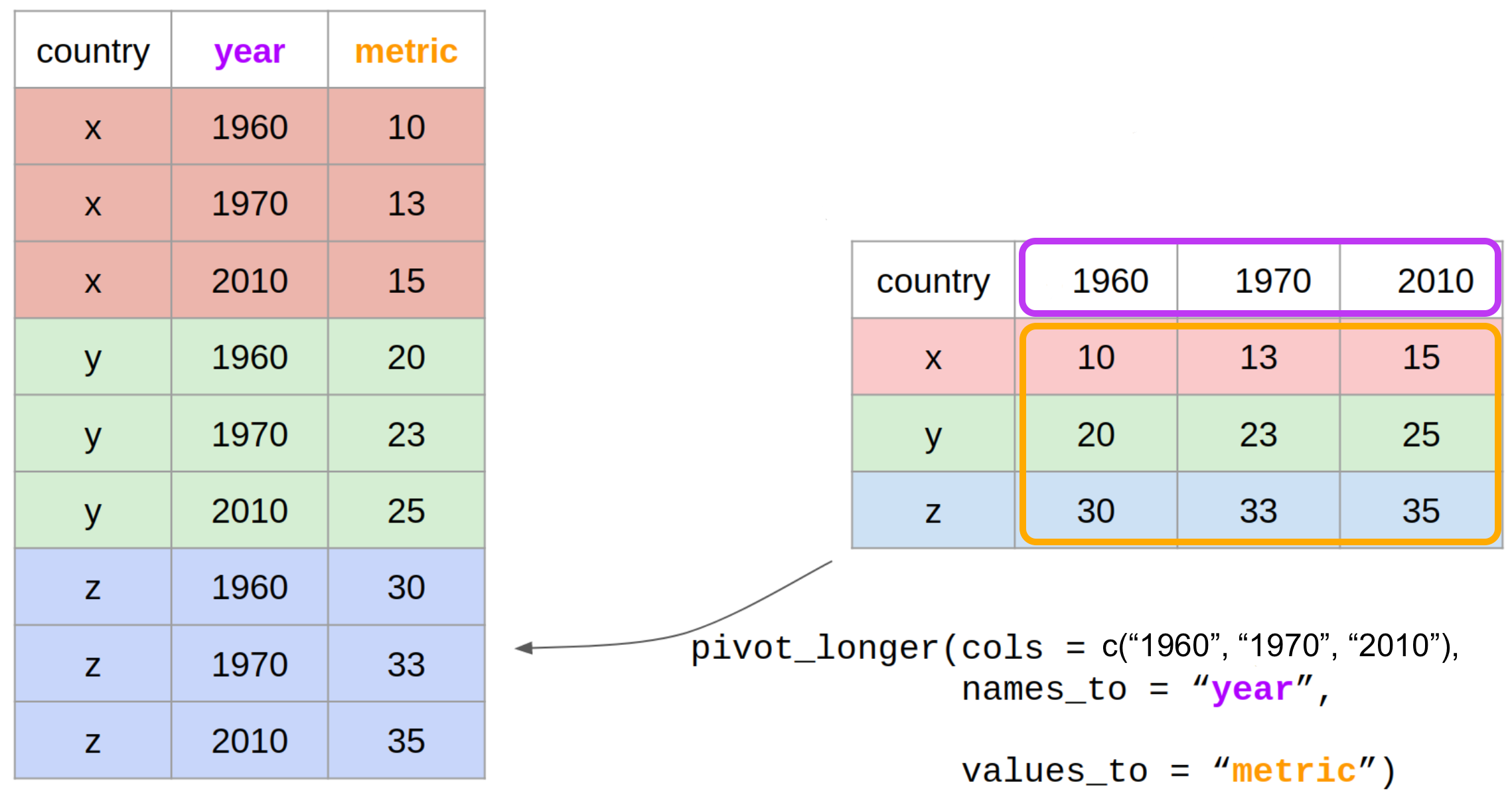
pivot_longer()

• data: data frame

• cols: columns to pivot into longer format (1960, 1970, 2010)

data |> pivot_longer(
    cols, 
    names_to = "name", 
    values_to = "value")

• So we are going to use a function pivot_longer().
• Like other functions in tidyverse, the first argument is again a data frame.
• then we give it the columns we want to pivot into the longer format

Source: https://tavareshugo.github.io/r-intro-tidyverse-gapminder/09-reshaping/index.html

pivot_longer()

• names_to: name of the column where column names of pivoted variables go (year)

data |> pivot_longer(
    cols, 
    names_to = "name", 
    values_to = "value")

Source: https://tavareshugo.github.io/r-intro-tidyverse-gapminder/09-reshaping/index.html

• and then we give the argument [names_to] the name of the column (in the transformed longer data) where column names of pivoted variables (in the original wider data) go, which is a character string.

pivot_longer()

• values_to: name of the column where data values in pivoted variables go (metric)

data |> pivot_longer(
    cols, 
    names_to = "name", 
    values_to = "value")

Source: https://tavareshugo.github.io/r-intro-tidyverse-gapminder/09-reshaping/index.html

• and finally we give the argument [values_to] the name of the column (in the transformed longer data) where data values of pivoted variables (in the original wider data) go, which is also a character string.
• So basically we are constructing two new variables in the new longer data set, and we are going to give their name as a character string, so they can be placed in the headers for those columns.

customers \(\rightarrow\) purchases

customers

# A tibble: 2 × 4
  customer_id item_1 item_2       item_3
        <dbl> <chr>  <chr>        <chr> 
1           1 bread  milk         banana
2           2 milk   toilet paper <NA>  

purchases <- customers |> pivot_longer(
    # variables item_1 to item_3 
    # to be pivoted into longer format 
    cols = item_1:item_3,
    
    # col name of the names of item_1:item_3
    # item_1 item_2 and item_3 
    names_to = "item_no",
    
    # col name of the values of item_1:item_3
    values_to = "item"
    )

purchases

# A tibble: 6 × 3
  customer_id item_no item        
        <dbl> <chr>   <chr>       
1           1 item_1  bread       
2           1 item_2  milk        
3           1 item_3  banana      
4           2 item_1  milk        
5           2 item_2  toilet paper
6           2 item_3  <NA>        

In customers data,

• Names item_1, item_2, item_3 are values of variable item_no in purchases

• Values bread, milk, etc are values of variable item in purchases

• Let’s see how the function actually works in the customers example.
• Suppose we start with the customers data set which is in a wider format.
• And we wanna pivot it into a longer format.
• the columns I wanna pivot are the ones that have information about the items that customers bought, which are item1, item 2, and item3.
• So I write item1:item3 (we can also use any helper function to select columns)
• OK Now, the column names item_1 item_2, item_3 should be in a new column in the transformed longer data set whose column name is called item_no.
• ANd the values in those three columns (the cells in the original data) should go into another new column in the in the transformed longer data set whose column name is called item that basically shows what the customers had purchased.
• So again the column names of the original wider data go into a new column called item_no
• and the values of the column names of the original wider data go into a new column called item.
• And I end up with a longer data set called purchases with 6 rows and 3 columns

Why Pivot?

• The next step of your analysis needs it.
• The new purchases data set and the prices data can now be joined together with the common key variable item.

prices <- read_csv("./data/sales/prices.csv")
prices

# A tibble: 5 × 2
  item         price
  <chr>        <dbl>
1 avocado       0.5 
2 banana        0.15
3 bread         1   
4 milk          0.8 
5 toilet paper  3   

purchases |> 
    left_join(prices) #<<

# A tibble: 6 × 4
  customer_id item_no item         price
        <dbl> <chr>   <chr>        <dbl>
1           1 item_1  bread         1   
2           1 item_2  milk          0.8 
3           1 item_3  banana        0.15
4           2 item_1  milk          0.8 
5           2 item_2  toilet paper  3   
6           2 item_3  <NA>         NA   

• Why do we want to pivot our data?
• Most likely, because the next step of your analysis needs it.
• Suppose we have another data set called prices as shown on the left that contains price of grocery items
• After pivoting our data, the new purchases data set and the prices data can now be joined together with the common key variable item.
• With the joined data set, we can further calculate total revenue for example.

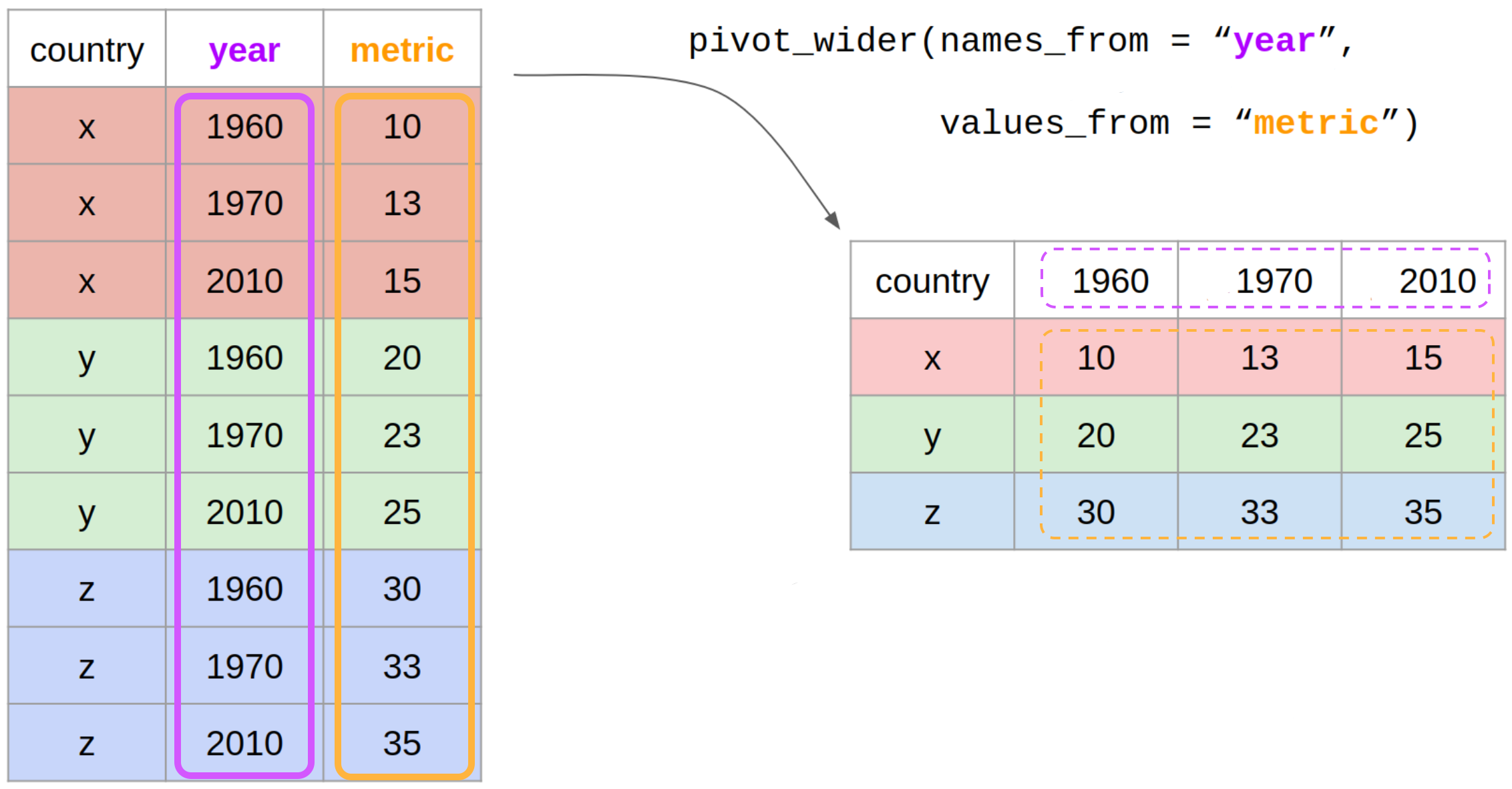
pivot_wider()

• data: data frame

• names_from: which column variable in the long format contains the what should be column names in the wide format (year)

data |> pivot_wider(
    names_from = column_variable_1, 
    values_from = column_variable_2)

Source: https://tavareshugo.github.io/r-intro-tidyverse-gapminder/09-reshaping/index.html

pivot_wider()

• data: data frame

• values_from: which column variable in the long format contains the what should be values in the new columns in the wide format (metric)

data |> pivot_wider(
    names_from = column_variable_1, 
    values_from = column_variable_2)

Source: https://tavareshugo.github.io/r-intro-tidyverse-gapminder/09-reshaping/index.html

purchases \(\rightarrow\) customers

purchases

# A tibble: 6 × 3
  customer_id item_no item        
        <dbl> <chr>   <chr>       
1           1 item_1  bread       
2           1 item_2  milk        
3           1 item_3  banana      
4           2 item_1  milk        
5           2 item_2  toilet paper
6           2 item_3  <NA>        

purchases |> 
    pivot_wider(              
        names_from = item_no, 
        values_from = item    
    ) 

# A tibble: 2 × 4
  customer_id item_1 item_2       item_3
        <dbl> <chr>  <chr>        <chr> 
1           1 bread  milk         banana
2           2 milk   toilet paper <NA>  

• All right. In fact we can also go back from a longer data to a wider data, which is the original data set we start with.
• data: data frame
• names_from: which column variable in the long format contains what should be column names in the wide format
• values_from: which column variable in the long format contains what should be (cell) values in the new columns in the wide format
• Notice that item_no and item are not quoted because they are variables that exist in our data frame purchases.
• We don’t construct new variables as we do when creating a data set in a longer format.
• OK. That’s pivoting, changing data set from wider to longer, or longer to wider format.

Source: FiveThirtyEight

17-tidyr

In lab.qmd ## Lab 17 section,

• Import trump.csv. Call it trump_data as below on the left.

• Use pivot_longer() to transform trump_data into the data set trump_longer on the right.

trump_data

# A tibble: 2,702 × 4
  subgroup date       approval disapproval
  <chr>    <date>        <dbl>       <dbl>
1 Voters   2020-10-04     44.7        52.2
2 Adults   2020-10-04     43.2        52.6
3 Adults   2020-10-03     43.2        52.6
4 Voters   2020-10-03     45.0        51.7
5 Adults   2020-10-02     43.3        52.4
6 Voters   2020-10-02     44.5        52.1
# ℹ 2,696 more rows

trump_longer <- ______________
    pivot_longer(
        cols = ____________,
        names_to = _______________,
        values_to = _______________
    ) 

# A tibble: 5,404 × 4
  subgroup date       rating_type rating_value
  <chr>    <date>     <chr>              <dbl>
1 Voters   2020-10-04 approval            44.7
2 Voters   2020-10-04 disapproval         52.2
3 Adults   2020-10-04 approval            43.2
4 Adults   2020-10-04 disapproval         52.6
5 Adults   2020-10-03 approval            43.2
6 Adults   2020-10-03 disapproval         52.6
# ℹ 5,398 more rows

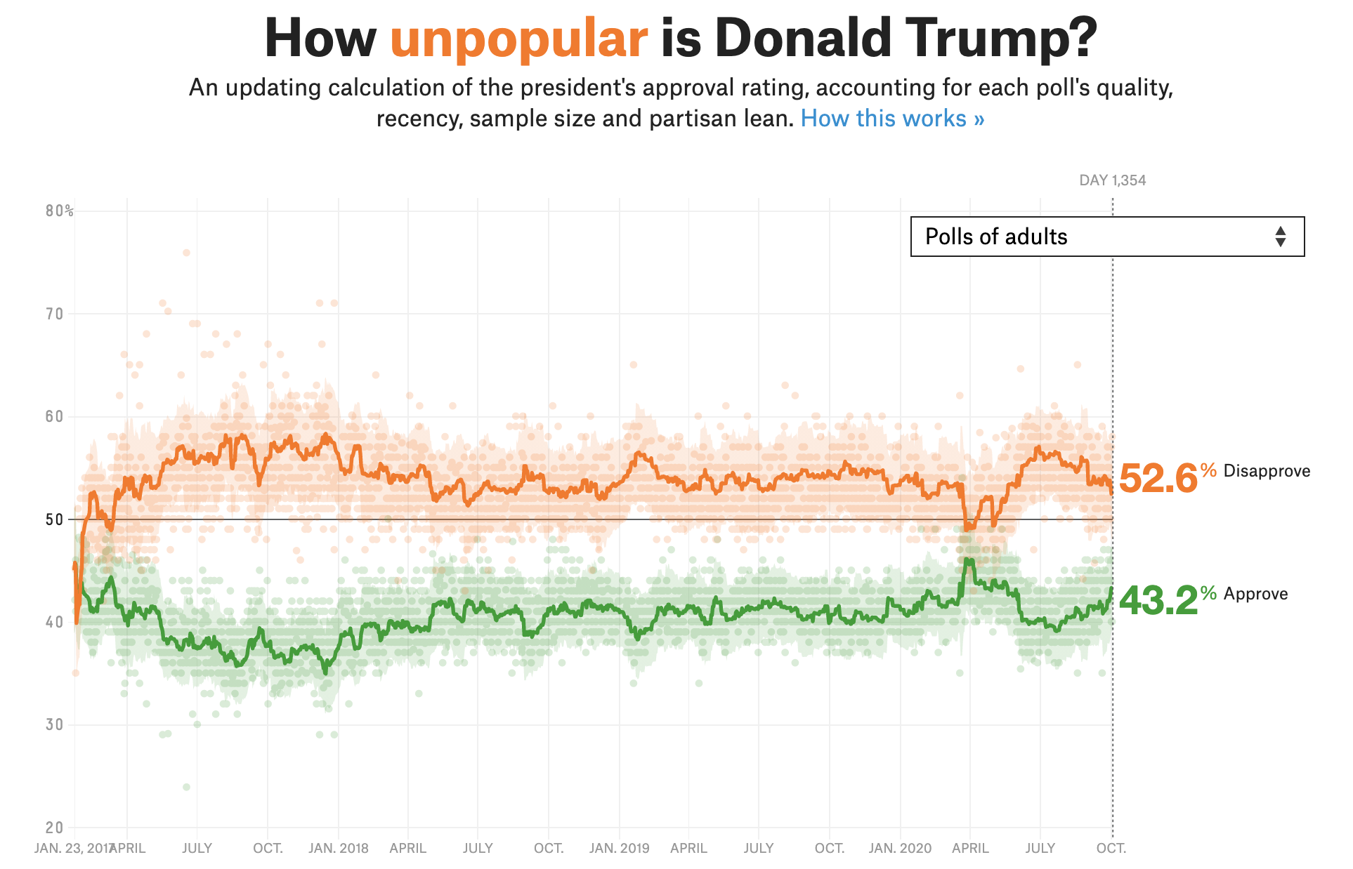
BONUS 💷: Use trump_longer to generate a plot like the one below.

Pivoting

pd.melt()

pd.pivot()

pd.melt()

import numpy as np
import pandas as pd

customers = pd.read_csv('./data/sales/customers.csv')
customers

   customer_id item_1        item_2  item_3
0            1  bread          milk  banana
1            2   milk  toilet paper     NaN

purchases = customers.melt(id_vars=['customer_id'], 
                           value_vars=['item_1', 'item_2', 'item_3'],
                           var_name='item_no', value_name='item')
purchases

   customer_id item_no          item
0            1  item_1         bread
1            2  item_1          milk
2            1  item_2          milk
3            2  item_2  toilet paper
4            1  item_3        banana
5            2  item_3           NaN

pd.pivot()

purchases

   customer_id item_no          item
0            1  item_1         bread
1            2  item_1          milk
2            1  item_2          milk
3            2  item_2  toilet paper
4            1  item_3        banana
5            2  item_3           NaN

purchases.pivot(index = "customer_id", columns = "item_no", values = "item")

item_no     item_1        item_2  item_3
customer_id                             
1            bread          milk  banana
2             milk  toilet paper     NaN