Basic R and Python

MATH/COSC 3570 Introduction to Data Science

Dr. Cheng-Han Yu
Department of Mathematical and Statistical Sciences
Marquette University

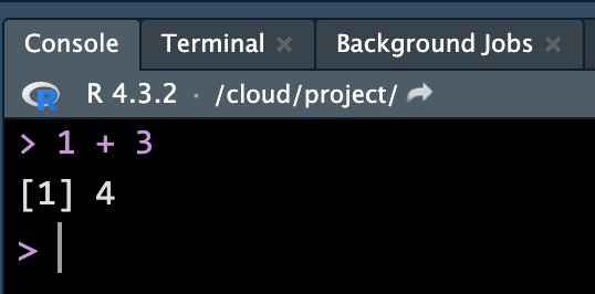
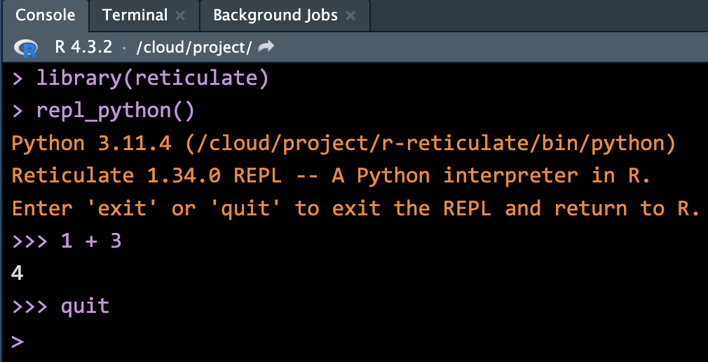
Run Code in Console

• reticulate::repl_python() to Python.

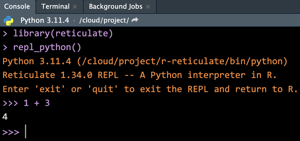
• quit or exit to switch back to R.

Arithmetic and Logical Operators

2 + 3 / (5 * 4) ^ 2

[1] 2.01

5 == 5.00

[1] TRUE

# 5 and 5L are of the same value too
# 5 is of type double; 5L is integer
5 == 5L

[1] TRUE

typeof(5L)

[1] "integer"

!TRUE == FALSE

[1] TRUE

2 + 3 / (5 * 4) ** 2

2.0075

5 == 5.00

True

5 == int(5)

True

type(int(5))

<class 'int'>

not True == False

True

repl_python()

Arithmetic and Logical Operators

Type coercion: When doing AND/OR comparisons, all nonzero values are treated as TRUE and 0 as FALSE.

-5 | 0

[1] TRUE

1 & 1

[1] TRUE

2 | 0

[1] TRUE

bool() converts nonzero numbers to True and zero to False

-5 | 0

-5

1 & 1

1

bool(2) | bool(0)

True

Math Functions

Math functions in R are built-in.

sqrt(144)

[1] 12

exp(1)

[1] 2.72

sin(pi/2)

[1] 1

log(32, base = 2)

[1] 5

abs(-7)

[1] 7

# R comment

Need to import math library in Python.

import math
math.sqrt(144)

12.0

math.exp(1)

2.718281828459045

math.sin(math.pi/2)

1.0

math.log(32, 2)

5.0

abs(-7)

7

# python comment

Variables and Assignment

Use <- to do assignment. Why

## we create an object, value 5, 
## and call it x, which is a variable
x <- 5
x

[1] 5

(x <- x + 6)

[1] 11

x == 5

[1] FALSE

log(x)

[1] 2.4

Use = to do assignment.

x = 5
x

5

x = x + 6
x

11

x == 5

False

math.log(x)

2.3978952727983707

Object Types

character, double, integer and logical.

typeof(5)

[1] "double"

typeof(5L)

[1] "integer"

typeof("I_love_data_science!")

[1] "character"

typeof(1 > 3)

[1] "logical"

is.double(5L)

[1] FALSE

str, float, int and bool.

type(5.0)

<class 'float'>

type(5)

<class 'int'>

type("I_love_data_science!")

<class 'str'>

type(1 > 3)

<class 'bool'>

type(5) is float

False

python long (long integers, they can also be represented in octal and hexadecimal)

R Data Structures

• Vector

• Factor

• List

• Matrix

• Data Frame

• Variable defined previously is a scalar value, or in fact a (atomic) vector of length one.

(Atomic) Vector

• To create a vector, use c(), short for concatenate or combine.
• All elements of a vector must be of the same type.

(dbl_vec <- c(1, 2.5, 4.5)) 

[1] 1.0 2.5 4.5

(int_vec <- c(1L, 6L, 10L))

[1]  1  6 10

## TRUE and FALSE can be written as T and F
(log_vec <- c(TRUE, FALSE, F))  

[1]  TRUE FALSE FALSE

(chr_vec <- c("pretty", "girl"))

[1] "pretty" "girl"  

## check how many elements in a vector
length(dbl_vec) 

[1] 3

## check a compact description of 
## any R data structure
str(dbl_vec) 

 num [1:3] 1 2.5 4.5

Sequence of Numbers

• Use : to create a sequence of integers.
• Use seq() to create a sequence of numbers of type double with more options.

(vec <- 1:5) 

[1] 1 2 3 4 5

typeof(vec)

[1] "integer"

# a sequence of numbers from 1 to 10 with increment 2
(seq_vec <- seq(from = 1, to = 10, by = 2))

[1] 1 3 5 7 9

typeof(seq_vec)

[1] "double"

Operations on Vectors

• We can do any operations on vectors as we do on a scalar variable (vector of length 1).

# Create two vectors
v1 <- c(3, 8)
v2 <- c(4, 100) 

## All operations happen element-wisely
# Vector addition
v1 + v2

[1]   7 108

# Vector subtraction
v1 - v2

[1]  -1 -92

# Vector multiplication
v1 * v2

[1]  12 800

# Vector division
v1 / v2

[1] 0.75 0.08

sqrt(v2)

[1]  2 10

Recycling of Vectors

• If we apply arithmetic operations to two vectors of unequal length, the elements of the shorter vector will be recycled to complete the operations.

v1 <- c(3, 8, 4, 5)
# The following 2 operations are the same
v1 * 2

[1]  6 16  8 10

v1 * c(2, 2, 2, 2)

[1]  6 16  8 10

v3 <- c(4, 11)
v1 + v3  ## v3 becomes c(4, 11, 4, 11) when doing the operation

[1]  7 19  8 16

Subsetting Vectors

• To extract element(s) in a vector, we use a pair of brackets [] with element indexing.
• The indexing starts with 1.

v1

[1] 3 8 4 5

v2

[1]   4 100

## The 3rd element
v1[3] 

[1] 4

v1[c(1, 3)]

[1] 3 4

v1[1:2]

[1] 3 8

## extract all except a few elements
## put a negative sign before the vector of 
## indices
v1[-c(2, 3)] 

[1] 3 5

Factor

• A vector of type factor can be ordered in a meaningful way. Create a factor by factor().

## Create a factor from a character vector using function factor()
(fac <- factor(c("med", "high", "low")))

[1] med  high low 
Levels: high low med

• It is a type of integer, not character. 😲 🙄

typeof(fac)  ## The type is integer.

[1] "integer"

str(fac)  ## The integers show the level each element in vector fac belongs to.

 Factor w/ 3 levels "high","low","med": 3 1 2

order_fac <- factor(c("med", "high", "low"),
                    levels = c("low", "med", "high"))
str(order_fac)

 Factor w/ 3 levels "low","med","high": 2 3 1

levels(fac) ## Each level represents an integer, ordered from the vector alphabetically.

List (Generic Vectors)

• Lists are different from (atomic) vectors: Elements can be of any type, including lists.

• Construct a list by using list().

## a list of 3 elements of different types
x_lst <- list(idx = 1:3, 
              "a", 
              c(TRUE, FALSE))

$idx
[1] 1 2 3

[[2]]
[1] "a"

[[3]]
[1]  TRUE FALSE

str(x_lst)

List of 3
 $ idx: int [1:3] 1 2 3
 $    : chr "a"
 $    : logi [1:2] TRUE FALSE

names(x_lst)

[1] "idx" ""    ""   

length(x_lst)

[1] 3

Subsetting a List

Return an element of a list

## subset by name (a vector)
x_lst$idx  

[1] 1 2 3

## subset by indexing (a vector)
x_lst[[1]]  

[1] 1 2 3

typeof(x_lst$idx)

[1] "integer"

Return a sub-list of a list

## subset by name (still a list)
x_lst["idx"]  

$idx
[1] 1 2 3

## subset by indexing (still a list)
x_lst[1]  

$idx
[1] 1 2 3

typeof(x_lst["idx"])

[1] "list"

• This is where we should pay more attention to. When we subset a list, it may return an element of the list, or it returns a sub-list of the list.
• Let’s see how it happens.
• This is our x_lst. We can subset a list by name or by indexing.
• Suppose we want the first element of the list, we can get it by its name using x_lst$idx.
• We can also obtain it by using indexing like x_lst[[1]] because we want the first element.
• Notice that the way we subset a list returns an integer vector, the real first element of the list, not a list.
• Let’s see another case on the right.
• We can also subset by name using single pair of brackets, and put the name inside the brackets.
• Or we can subset by indexing, again using single pair of brackets.
• And you see what happened? The way we subset a list here returns a sub-list, not the element itself.
• So please be careful when subsetting a list.
• If you want a vector, use these ways. If you want to keep it as a list, use these ways.

pepper packet pepper shaker

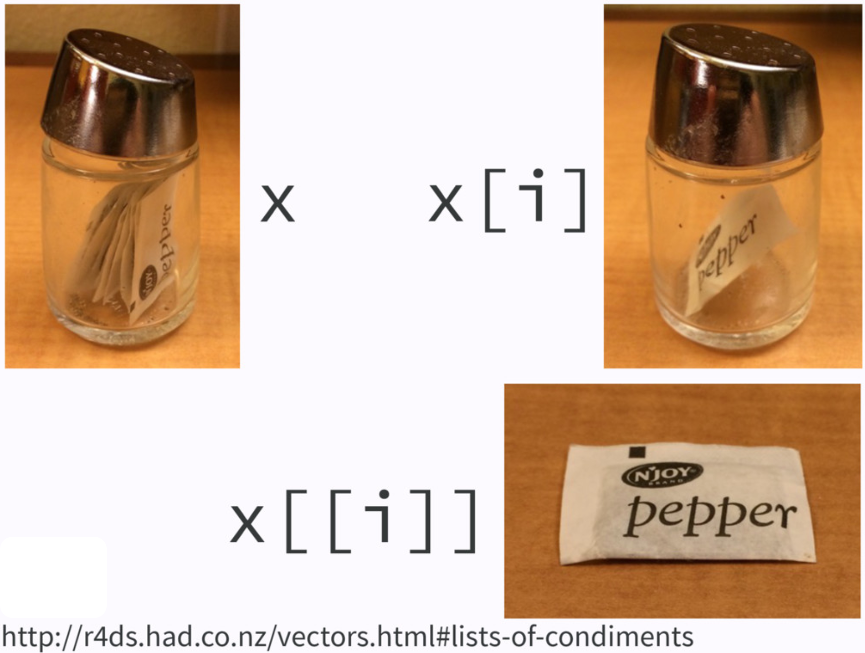
If list x is a train carrying objects, then x[[5]] is the object in car 5; x[4:6] is a train of cars 4-6.

— @RLangTip, https://twitter.com/RLangTip/status/268375867468681216

Matrix

• A matrix is a two-dimensional analog of a vector with attribute dim.
• Use command matrix() to create a matrix.

## Create a 3 by 2 matrix called mat
(mat <- matrix(data = 1:6, nrow = 3, ncol = 2)) 

     [,1] [,2]
[1,]    1    4
[2,]    2    5
[3,]    3    6

dim(mat); nrow(mat); ncol(mat)

[1] 3 2

[1] 3

[1] 2

     [,1] [,2]
[1,]    1    2
[2,]    3    4
[3,]    5    6

$dim
[1] 3 2

Subsetting a Matrix

• Use the same indexing approach as vectors on rows and columns.
• Use comma , to separate row and column index.
• mat[2, 2] extracts the element of the second row and second column.

mat

     [,1] [,2]
[1,]    1    4
[2,]    2    5
[3,]    3    6

## all rows and 2nd column
## leave row index blank
## specify 2 in coln index
mat[, 2]

[1] 4 5 6

## 2nd row and all columns
mat[2, ] 

[1] 2 5

## The 1st and 3rd rows and the 1st column
mat[c(1, 3), 1] 

[1] 1 3

Binding Matrices

• cbind() (binding matrices by adding columns)

• rbind() (binding matrices by adding rows)

• When matrices are combined by columns (rows), they should have the same number of rows (columns).

mat

     [,1] [,2]
[1,]    1    4
[2,]    2    5
[3,]    3    6

mat_c <- matrix(data = c(7,0,0,8,2,6), 
                nrow = 3, ncol = 2)
## should have the same number of rows
cbind(mat, mat_c)  

     [,1] [,2] [,3] [,4]
[1,]    1    4    7    8
[2,]    2    5    0    2
[3,]    3    6    0    6

mat_r <- matrix(data = 1:4, 
                nrow = 2, 
                ncol = 2)
## should have the same number of columns
rbind(mat, mat_r)  

     [,1] [,2]
[1,]    1    4
[2,]    2    5
[3,]    3    6
[4,]    1    3
[5,]    2    4

Data Frame: The Most Common Way of Storing Datasets

• A data frame is of type list of equal-length vectors, having a 2-dimensional structure.
• More general than matrix: Different columns can have different types.
• Use data.frame() that takes named vectors as input “element”.

## data frame w/ an dbl column named age
## and char column named gender.
(df <- data.frame(age = c(19, 21, 40), 
                  gen = c("m", "f", "m")))

  age gen
1  19   m
2  21   f
3  40   m

## a data frame has a list structure
str(df)  

'data.frame':   3 obs. of  2 variables:
 $ age: num  19 21 40
 $ gen: chr  "m" "f" "m"

## must set column names
## or they are ugly and non-recognizable
data.frame(c(19, 21, 40), c("m", "f", "m")) 

  c.19..21..40. c..m....f....m..
1            19                m
2            21                f
3            40                m

Properties of Data Frames

Data frame has properties of matrix and list.

names(df)  ## df as a list

[1] "age" "gen"

colnames(df)  ## df as a matrix

[1] "age" "gen"

length(df) ## df as a list

[1] 2

ncol(df) ## df as a matrix

[1] 2

dim(df) ## df as a matrix

[1] 3 2

## rbind() and cbind() can be used on df
df_r <- data.frame(age = 10, 
                   gen = "f")
rbind(df, df_r)

  age gen
1  19   m
2  21   f
3  40   m
4  10   f

df_c <- 
    data.frame(col = c("red","blue","gray"))
(df_new <- cbind(df, df_c))

  age gen  col
1  19   m  red
2  21   f blue
3  40   m gray

Subsetting a Data Frame

Can use either list or matrix subsetting methods.

df_new

  age gen  col
1  19   m  red
2  21   f blue
3  40   m gray

## Subset rows
df_new[c(1, 3), ]

  age gen  col
1  19   m  red
3  40   m gray

## select the row where age == 21
df_new[df_new$age == 21, ]

  age gen  col
2  21   f blue

## Subset columns
## like a list
df_new$age

[1] 19 21 40

df_new[c("age", "gen")]

  age gen
1  19   m
2  21   f
3  40   m

## like a matrix
df_new[, c("age", "gen")]

  age gen
1  19   m
2  21   f
3  40   m

  age gen  col
1  19   m  red
3  40   m gray

'data.frame':   3 obs. of  1 variable:
 $ age: num  19 21 40

 num [1:3] 19 21 40

05-R Data Type Summary

In lab.qmd Lab 5,

• Create R objects vector v1, factor f2, list l3, matrix m4 and data frame d5.

• Check typeof() and class() of those objects, and create a list having the output below.

v1 <- __________
f2 <- __________
l3 <- __________
m4 <- __________
d5 <- __________
v <- c(type = typeof(v1), class = class(v1))
f <- c(type = __________, class = _________)
l <- c(type = __________, class = _________)
m <- c(type = __________, class = _________)
d <- c(type = __________, class = _________)
____(vec    =   v,
     ______ = ___,
     ______ = ___,
     ______ = ___,
     ______ = ___)

$vec
     type     class 
 "double" "numeric" 

$fac
     type     class 
"integer"  "factor" 

$lst
  type  class 
"list" "list" 

$mat
     type    class1    class2 
"integer"  "matrix"   "array" 

$df
        type        class 
      "list" "data.frame" 

Python Data Structures

• List

• Tuple

• Dictionary

Python Lists

• Python has numbers and strings, but no built-in vector structure.
• To create a sequence type of structure, we can use a list that can save several elements in an single object.
• To create a list in Python, we use [].

lst_num = [0, 2, 4] 
lst_num

[0, 2, 4]

type(lst_num)

<class 'list'>

len(lst_num)

3

List elements can have different types!

lst = ['data', 'math', 34, True]
lst

['data', 'math', 34, True]

Subsetting Lists

• Indexing in Python always starts at 0!
• 0: the 1st element

lst

['data', 'math', 34, True]

lst[0]

'data'

type(lst[0]) ## not a list

<class 'str'>

• -1: the last element

lst[-2]

34

• [a:b]: the (a+1)-th to b-th elements

lst[1:4]

['math', 34, True]

type(lst[1:4]) ## a list

<class 'list'>

• [a:]: elements from the (a+1)-th to the last

lst[2:]

[34, True]

What does lst[0:1] return? Is it a list?

What does lst[0:1] return? Is it a list?

Lists are Mutable

Lists are changed in place!

lst[1]

'math'

lst[1] = "stats"
lst

['data', 'stats', 34, True]

lst[2:] = [False, 77]
lst

['data', 'stats', False, 77]

If we change any element value in a list, the list itself will be changed as well.

List Operations and Methods list.method()

## Concatenation
lst_num + lst

[0, 2, 4, 'data', 'stats', False, 77]

## Repetition
lst_num * 3 

[0, 2, 4, 0, 2, 4, 0, 2, 4]

## Membership
34 in lst

False

## Appends "cat" to lst
lst.append("cat")
lst

['data', 'stats', False, 77, 'cat']

## Removes and returns last object from list
lst.pop()

'cat'

lst

['data', 'stats', False, 77]

## Removes object from list
lst.remove("stats")
lst

['data', False, 77]

## Reverses objects of list in place
lst.reverse()
lst

[77, False, 'data']

This is a common syntax in Python. We start with a Pyhton object of some type, then type dot followed by any method specifically for this particular data type or structure for operations. list.pop(index)

Tuples

• Tuples work exactly like lists except they are immutable, i.e., they can’t be changed in place.

• To create a tuple, we use ().

tup = ('data', 'math', 34, True)
tup

('data', 'math', 34, True)

type(tup)

<class 'tuple'>

len(tup)

4

tup[2:]

(34, True)

tup[-2]

34

tup[1] = "stats"  ## does not work!
# TypeError: 'tuple' object does not support item assignment

tup

('data', 'math', 34, True)

‘tuple’ object does not support item assignment

Tuples Functions and Methods

# Converts a list into tuple
tuple(lst_num)

(0, 2, 4)

# number of occurance of "data"
tup.count("data")

1

# first index of "data"
tup.index("data")

0

Note

Lists have more methods than tuples because lists are more flexible.

Dictionaries

• A dictionary consists of key-value pairs.

• A dictionary is mutable, i.e., the values can be changed in place and more key-value pairs can be added.

• To create a dictionary, we use {'key': value}.

• The value can be accessed by the key in the dictionary.

dic = {'Name': 'Ivy', 'Age': 7, 'Class': 'First'}

dic['Age']

7

dic['age']  ## does not work

dic['Age'] = 9
dic['Class'] = 'Third'
dic

{'Name': 'Ivy', 'Age': 9, 'Class': 'Third'}

Properties of Dictionaries

• Python will use the last assignment!

dic1 = {'Name': 'Ivy', 'Age': 7, 'Name': 'Liya'}
dic1['Name']

'Liya'

• Keys are unique and immutable.

• A key can be a tuple, but CANNOT be a list.

## The first key is a tuple!
dic2 = {('First', 'Last'): 'Ivy Lee', 'Age': 7}
dic2[('First', 'Last')]

'Ivy Lee'

## does not work
dic2 = {['First', 'Last']: 'Ivy Lee', 'Age': 7}
dic2[['First', 'Last']]

Dictionary Methods

{'Name': 'Ivy', 'Age': 9, 'Class': 'Third'}

dic.keys() ## Returns list of dictionary dict's keys

dict_keys(['Name', 'Age', 'Class'])

dic.values() ## Returns list of dictionary dict's values

dict_values(['Ivy', 9, 'Third'])

dic.items() ## Returns a list of dict's (key, value) tuple pairs

dict_items([('Name', 'Ivy'), ('Age', 9), ('Class', 'Third')])

## Adds dictionary dic2's key-values pairs in to dic
dic2 = {'Gender': 'female'}
dic.update(dic2)
dic

{'Name': 'Ivy', 'Age': 9, 'Class': 'Third', 'Gender': 'female'}

## Removes all elements of dictionary dict
dic.clear()
dic

{}

06-Python Data Structure

In lab.qmd Lab 6,

• Create a Python list and dictionary similar to the R list below.

x_lst <- list(idx = 1:3, 
              "a", 
              c(TRUE, FALSE))

Remember to create Python code chunk

```{Python}
#| echo: true
#| eval: false
#| code-line-numbers: false

```

Any issue of this Python chunk?

Commit and Push your work once you are done.

Python Data Structures for Data Science

• Python built-in data structures are not specifically for data science.

• To use more data science friendly functions and structures, such as array or data frame, Python relies on packages NumPy and pandas.

Installing NumPy and pandas*

In your lab-yourusername project, run

library(reticulate)
virtualenv_create("myenv")

Go to Tools > Global Options > Python > Select > Virtual Environments

Installing NumPy and pandas*

You may need to restart R session. Do it, and in the new R session, run

library(reticulate)
py_install(c("numpy", "pandas", "matplotlib"))

Run the following Python code, and make sure everything goes well.

import numpy as np
import pandas as pd
v1 = np.array([3, 8])
v1

array([3, 8])

df = pd.DataFrame({"col": ['red', 'blue', 'green']})
df

     col
0    red
1   blue
2  green

Descriptive Statistics (MATH 4720)

• Central Tendency and Variability

• Data Summary

Central Tendency: Mean and Median

data <- c(3,12,56,9,230,22)
mean(data)

[1] 55.3

median(data)  

[1] 17

data = np.array([3,12,56,9,230,22])
type(data)

<class 'numpy.ndarray'>

np.mean(data)

55.333333333333336

np.median(data)

17.0

• The (arithmetic) mean or average is adding up all of the values, then dividing by the total number of them.
• Mean balances data Values.
• The median is the middle value when data values are arranged from the lowest to highest.
• Mean is sensitive to extreme values (outliers).

Variation

quantile(data, c(0.25, 0.5, 0.75)) 

  25%   50%   75% 
 9.75 17.00 47.50 

var(data)

[1] 7677

sd(data)

[1] 87.6

summary(data)

   Min. 1st Qu.  Median    Mean 3rd Qu.    Max. 
    3.0     9.8    17.0    55.3    47.5   230.0 

np.quantile(data,  [0.25, 0.5, 0.75])

array([ 9.75, 17.  , 47.5 ])

np.var(data, ddof = 1)

7676.666666666666

np.std(data, ddof = 1)

87.61658899242008

df = pd.Series(data)
df.describe()

count      6.000000
mean      55.333333
std       87.616589
min        3.000000
25%        9.750000
50%       17.000000
75%       47.500000
max      230.000000
dtype: float64

• p-th percentile: a data value such that at most \(p\%\) of the data values are below it and at most \((1−p)\%\) of the values are above it.
• First Quartile (Q1): the 25-th percentile
• Second Quartile (Q2): the 50-th percentile (Median)
• Third Quartile (Q3): the 75-th percentile
• Interquartile Range (IQR): Q3 - Q1

IQR(data)

q75, q25 = np.percentile(data, [75 ,25])
q75 - q25

Delta Degrees of Freedom.

Basic Plotting

• Scatter Plot

• Boxplot

• Histogram

• Bar Chart

• Pie Chart

• 2D Imaging

• 3D Plotting

R plot()

mtcars[1:15, 1:4]

                    mpg cyl disp  hp
Mazda RX4          21.0   6  160 110
Mazda RX4 Wag      21.0   6  160 110
Datsun 710         22.8   4  108  93
Hornet 4 Drive     21.4   6  258 110
Hornet Sportabout  18.7   8  360 175
Valiant            18.1   6  225 105
Duster 360         14.3   8  360 245
Merc 240D          24.4   4  147  62
Merc 230           22.8   4  141  95
Merc 280           19.2   6  168 123
Merc 280C          17.8   6  168 123
Merc 450SE         16.4   8  276 180
Merc 450SL         17.3   8  276 180
Merc 450SLC        15.2   8  276 180
Cadillac Fleetwood 10.4   8  472 205

plot(x = mtcars$mpg, y = mtcars$hp, 
     xlab  = "Miles per gallon", 
     ylab = "Horsepower", 
     main = "Scatter plot", 
     col = "red", 
     pch = 5, las = 1)

Argument pch

• The defualt is pch = 1

Python matplotlib.pyplot

mtcars = pd.read_csv('./data/mtcars.csv')
mtcars.iloc[0:15,0:4]

     mpg  cyl   disp   hp
0   21.0    6  160.0  110
1   21.0    6  160.0  110
2   22.8    4  108.0   93
3   21.4    6  258.0  110
4   18.7    8  360.0  175
5   18.1    6  225.0  105
6   14.3    8  360.0  245
7   24.4    4  146.7   62
8   22.8    4  140.8   95
9   19.2    6  167.6  123
10  17.8    6  167.6  123
11  16.4    8  275.8  180
12  17.3    8  275.8  180
13  15.2    8  275.8  180
14  10.4    8  472.0  205

import matplotlib.pyplot as plt
plt.scatter(x = mtcars.mpg, 
            y = mtcars.hp, 
            color = "r")
plt.xlabel("Miles per gallon")
plt.ylabel("Horsepower")
plt.title("Scatter plot")

R Subplots

par(mfrow = c(1, 2))
plot(x = mtcars$mpg, y = mtcars$hp, xlab = "mpg")
plot(x = mtcars$mpg, y = mtcars$wt, xlab = "mpg")

Python Subplots

• The command plt.scatter() is used for creating one single plot.

• If multiple subplots are wanted in one single call, one can use plt.subplots()

fig, (ax1, ax2) = plt.subplots(1, 2)
ax1.scatter(x = mtcars.mpg, y = mtcars.hp)
ax2.scatter(x = mtcars.mpg, y = mtcars.wt)
ax1.set_xlabel("mpg")
ax2.set_xlabel("mpg")

R boxplot()

boxplot(mpg ~ cyl, 
        data = mtcars, 
        col = c("blue", "green", "red"), 
        las = 1, 
        horizontal = TRUE,
        xlab = "Miles per gallon", 
        ylab = "Number of cylinders")

• Visualizing relationships between numerical and categorical data, we can check side-by-side boxplots.
• For example, if we want to check the data variation of (miles per gallon) for each number of cylinder, we can use boxplot() function.
• And inside the function, we use the formula mpg ~ cyl, and specify the dataset.
• That is basically it. The rest of arguments are decorating your plot. They are optional.

Python boxplot()

cyl_num = np.unique(mtcars.cyl)
cyl_list = []
cyl_list.append(mtcars[mtcars.cyl == cyl_num[0]].mpg)
cyl_list.append(mtcars[mtcars.cyl == cyl_num[1]].mpg)
cyl_list.append(mtcars[mtcars.cyl == cyl_num[2]].mpg)

import matplotlib.pyplot as plt
plt.boxplot(cyl_list, vert=False, tick_labels=[4, 6, 8])

plt.xlabel("Miles per gallon")
plt.ylabel("Number of cylinders")

R hist()

• hist() decides the class intervals/with based on breaks. If not provided, R chooses one.

hist(mtcars$wt, 
     breaks = 20, 
     col = "#003366", 
     border = "#FFCC00", 
     xlab = "weights", 
     main = "Histogram of weights",
     las = 1)

• Besides color names, you can also use hex number to specify colors. Pretty handy.

Python hist()

## by default bins=10
plt.hist(mtcars.wt, 
         bins = 20, 
         color="#003366",
         edgecolor="#FFCC00")
plt.xlabel("weights")
plt.title("Histogram of weights")

R barplot()

(counts <- table(mtcars$gear)) 

 3  4  5 
15 12  5 

my_bar <- barplot(counts, 
                  main = "Car Distribution", 
                  xlab = "Number of Gears", 
                  las = 1)
text(x = my_bar, y = counts - 0.8, 
     labels = counts, 
     cex = 0.8)

Python barplot()

count_py = mtcars.value_counts('gear')
count_py

gear
3    15
4    12
5     5
Name: count, dtype: int64

plt.bar(["3", "4", "5"], count_py)
plt.xlabel("Number of Gears")
plt.title("Car Distribution")

R pie()

(percent <- round(counts / sum(counts) * 100, 2))

   3    4    5 
46.9 37.5 15.6 

(labels <- paste0(3:5, " gears: ", percent, "%"))

[1] "3 gears: 46.88%" "4 gears: 37.5%"  "5 gears: 15.62%"

pie(x = counts, labels = labels,
    main = "Pie Chart", 
    col = 2:4, 
    radius = 1)

• Pie charts are used for categorical variables, especially when we want to know percentage of each category.
• The first argument is the frequency table, and you can add labels to each category.

Python pie()

percent = round(count_py / sum(count_py) * 100, 2)
texts = (percent.index.astype(str) + " gears: " + percent.astype(str) + "%").tolist()

plt.pie(count_py, labels = texts, colors = ['r', 'g', 'b'])

plt.title("Pie Charts")

R 2D Imaging: image()

• The image() function displays the values in a matrix using color.

matrix(1:30, 6, 5)

     [,1] [,2] [,3] [,4] [,5]
[1,]    1    7   13   19   25
[2,]    2    8   14   20   26
[3,]    3    9   15   21   27
[4,]    4   10   16   22   28
[5,]    5   11   17   23   29
[6,]    6   12   18   24   30

image(matrix(1:30, 6, 5))

In Python,

matrix = np.arange(1, 31).reshape(5, 6)
plt.imshow(matrix, cmap="viridis", origin="lower")
plt.colorbar()
plt.show()

R fields::image.plot()

library(fields)
str(volcano)

 num [1:87, 1:61] 100 101 102 103 104 105 105 106 107 108 ...

image.plot(volcano)

 num [1:87, 1:61] 100 101 102 103 104 105 105 106 107 108 ...

R 2D Imaging Example: Volcano

R 3D scatter plot: scatterplot3d()

library(scatterplot3d)
scatterplot3d(x = mtcars$wt, 
              y = mtcars$disp, 
              z = mtcars$mpg, 
              main = "3D Scatter Plot", 
              xlab = "Weights", 
              ylab = "Displacement",
              zlab = "Miles per gallon", 
              pch = 16, 
              color = "steelblue")

In Python,

fig = plt.figure()
ax = fig.add_subplot(projection='3d')
ax.scatter(mtcars['wt'], mtcars['disp'], mtcars['mpg'], c='steelblue', marker='o')
ax.set_title("3D Scatter Plot")
ax.set_xlabel("Weights")
ax.set_ylabel("Displacement")
ax.set_zlabel("Miles per gallon")
plt.show()

R Perspective Plot: persp()

par(mar = c(0,0,0,0))
# Exaggerate the relief
z <- 2 * volcano      
# 10 meter spacing (S to N)
x <- 10 * (1:nrow(z))   
# 10 meter spacing (E to W)
y <- 10 * (1:ncol(z))   
par(bg = "slategray")
persp(x, y, z, theta = 135, phi = 30, 
      col = "green3", scale = FALSE,
      ltheta = -120, shade = 0.75, 
      border = NA, box = FALSE)

In Python,

volcano = pd.read_csv("./slides/data/volcano.csv", index_col=0)
volcano = volcano.values
z = 2 * volcano
x = np.arange(1, z.shape[0] + 1) * 10
y = np.arange(1, z.shape[1] + 1) * 10  
X, Y = np.meshgrid(y, x)
fig = plt.figure()
ax = fig.add_subplot(projection='3d', facecolor="slategray")
ax.plot_surface(X, Y, z, cmap="Greens", edgecolor="none", shade=True, alpha=0.9)
plt.show()

• You can also generate a so-called perspective plot using the function persp().
• I don’t use the function often. You can try it with different argument values, and see how it changes.

07-Plotting

In lab.qmd ## Lab 7,

• For the mtcars data, use R or Python to

  • make a scatter plot of miles per gallon vs. weight. Decorate your plot using arguments, col, pch, xlab, etc.

  • create a histogram of 1/4 mile time. Make it beautiful!

• Commit and Push your work once you are done.

import pandas as pd
import matplotlib.pyplot as plt
mtcars = pd.read_csv('./data/mtcars.csv')

Resources

• The R Graph Gallery
• matplotlib

We will talk about data visualization in detail soon!

https://stackoverflow.com/questions/43482191/matplotlib-axes-plot-vs-pyplot-plot